
Naive Bayes Classifier Explained: How It Works with Examples
Learn how the Naive Bayes classifier works: Bayes' theorem, the independence assumption, Laplace smoothing, a worked example and a Python spam filter.
 Nov 12, 2026Published
19 min readReading time
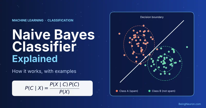
The Naive Bayes classifier is a supervised learning algorithm that predicts the class of a new example by applying Bayes’ theorem with one simplifying assumption: once the class is known, every feature is treated as independent of the others. Real data rarely behaves that way, which is where the word “naive” comes from. Even so, the algorithm is fast, works with small training sets, and remains a strong baseline for text problems such as spam filtering.
In supervised learning, a model learns from labeled examples. Naive Bayes is a classification method: it assigns an input to one of several discrete classes, such as “spam” or “not spam”. Rather than drawing a boundary between classes, it estimates how probable each class is for the input and picks the most probable one.
By the end of this guide you will be able to compute a Naive Bayes prediction by hand, explain Laplace smoothing, choose between the three common variants, and build a working spam classifier with Scikit-learn.
Key terms used in this guide
- Class (label): the category we want to predict, for example spam or ham (legitimate email).
- Feature: a measurable property of an example, such as whether the word “win” appears.
- Prior: the probability of a class before looking at any features.
- Likelihood: how probable the observed features are if a given class is true.
- Posterior: the updated probability of a class after seeing the features.
Understanding Bayes’ Theorem
Bayes’ theorem describes how to update a belief when new evidence arrives. For two events A and B it states:
| P(A | B) = | P(B | A) × P(A) |
| P(B) |
- P(A | B) is the posterior: the probability of A after observing B. The vertical bar reads “given”.
- P(B | A) is the likelihood: how likely B is if A is true.
- P(A) is the prior: how likely A was before seeing B.
- P(B) is the evidence: how likely B is overall, across all possibilities for A.
A Quick Numerical Example
Suppose 40% of emails are spam. The word “win” appears in 70% of spam emails and in 5% of legitimate emails. An email arrives containing “win”. How likely is it to be spam?
- Prior: P(spam) = 0.40 and P(ham) = 0.60.
- Likelihoods: P(win | spam) = 0.70 and P(win | ham) = 0.05.
- Evidence: P(win) = 0.70 × 0.40 + 0.05 × 0.60 = 0.28 + 0.03 = 0.31.
- Posterior: P(spam | win) = 0.28 / 0.31 ≈ 0.90.
Seeing the word raised our belief that the email is spam from 40% to about 90%. Figure 1 shows the same flow.
From Bayes’ Theorem to Classification
To classify, let A be the class y and B be the observed features x = (x1, …, xn). The theorem becomes P(y | x) = P(x | y) × P(y) / P(x). The denominator P(x) is the same for every class, so when we only need to rank classes we can ignore it and compare P(x | y) × P(y).
Why Is It Called Naive Bayes?
The hard part is P(x | y), the probability of seeing an entire combination of features given the class. With n binary features, describing that joint distribution fully takes 2n − 1 numbers per class. For a 1,000-word vocabulary that is far more combinations than any dataset can cover.
Naive Bayes removes the problem with the conditional independence assumption: given the class, each feature is assumed to be independent of every other feature. The joint probability then factors into a product of simple per-feature probabilities, and only n numbers per class are needed.
The assumption is “naive” because it is usually false. In spam email, “free” and “prize” tend to appear together, so they are not independent even within the spam class. The model ignores that link and treats each word as separate evidence.
Why It Still Works
Classification only needs the correct class to receive the highest score; it does not need accurate probabilities. Domingos and Pazzani (1997) showed that the classifier can be optimal under zero-one loss even when the independence assumption is clearly violated. The cost is that the predicted probabilities are often too extreme, so treat predict_proba output as a ranking signal rather than a calibrated probability, as the Scikit-learn documentation also advises.
How the Naive Bayes Algorithm Works
The algorithm has a training phase that only counts and averages, and a prediction phase that scores each class.
- Collect labeled data and convert each example into features.
- Estimate the priors P(y) from the share of training examples in each class.
- Estimate the likelihoods P(xi | y) for every feature and class, applying smoothing so no probability is zero.
- Score a new example for each class by combining its prior with the likelihoods of its features.
- Predict the class with the highest score.
Mathematical Explanation and Formula
Applying the Independence Assumption
Conditional independence means that, given the class y, knowing one feature tells us nothing extra about another:
P(x1, x2, …, xn | y) = ∏i=1n P(xi | y)
Substituting this into Bayes’ theorem and dropping the constant denominator gives the Naive Bayes decision rule:
ŷ = argmaxy P(y) ∏i=1n P(xi | y)
Here ŷ is the predicted class, “argmax” means “the class that gives the largest value”, and ∏ means “multiply all of these terms”.
Working in Log Space
Multiplying hundreds of probabilities, each below 1, quickly produces numbers too small for a computer to store, an effect called underflow. Because the logarithm is increasing, taking logs does not change which class wins, and it turns the product into a sum:
ŷ = argmaxy [ log P(y) + ∑i=1n log P(xi | y) ]
Scikit-learn does this internally, which is why fitted models expose attributes such as class_log_prior_ and feature_log_prob_.
Laplace Smoothing
Suppose the word “win” never appeared in any legitimate email in the training data. Then P(win | ham) = 0, and because the likelihoods are multiplied, any new email containing “win” would get a ham score of exactly zero, no matter how business-like the rest of it is. One unseen word would veto an entire class.
Laplace smoothing (also called additive smoothing) fixes this by adding a small pseudo-count α to every word count:
| P(w | c) = | Nw,c + α |
| Nc + αV |
- Nw,c is how many times word w appears in training documents of class c.
- Nc is the total number of word occurrences in class c.
- V is the vocabulary size, the number of distinct words. Adding αV to the denominator keeps the probabilities summing to 1.
- α = 1 is classic Laplace smoothing. Values between 0 and 1 are sometimes called Lidstone smoothing. Scikit-learn exposes it as the
alphaparameter, with a default of 1.0.
Step-by-Step Classification Example
Let’s classify an email by hand. Imagine a tiny training set of 4 spam emails and 6 ham emails, with a vocabulary of V = 5 words. The table shows how often each word occurred in each class.
| Word | Count in spam | Count in ham |
|---|---|---|
| free | 8 | 2 |
| win | 6 | 0 |
| prize | 4 | 1 |
| meeting | 1 | 15 |
| report | 1 | 12 |
| Total words | 20 | 30 |
The new email to classify contains the words “meeting report win”. It looks like a business message with one suspicious word.
Step 1: Compute the priors
P(spam) = 4 / 10 = 0.40 and P(ham) = 6 / 10 = 0.60.
Step 2: Try it without smoothing
Using raw frequencies, P(win | ham) = 0 / 30 = 0. The scores are:
- Spam: 0.40 × (1/20) × (1/20) × (6/20) = 0.0003
- Ham: 0.60 × (15/30) × (12/30) × 0 = 0
The model would label this email spam only because a single zero erased the ham class. That is the failure Laplace smoothing prevents.
Step 3: Apply Laplace smoothing (α = 1)
Add 1 to every count and add V = 5 to each class total, so the denominators become 25 for spam and 35 for ham.
| Word | P(word | spam) | P(word | ham) |
|---|---|---|
| meeting | (1 + 1) / 25 = 0.080 | (15 + 1) / 35 ≈ 0.457 |
| report | (1 + 1) / 25 = 0.080 | (12 + 1) / 35 ≈ 0.371 |
| win | (6 + 1) / 25 = 0.280 | (0 + 1) / 35 ≈ 0.029 |
Step 4: Score each class
- Spam: 0.40 × 0.080 × 0.080 × 0.280 ≈ 0.000717
- Ham: 0.60 × 0.457 × 0.371 × 0.0286 ≈ 0.002911
Step 5: Normalize and decide
The total is 0.000717 + 0.002911 = 0.003628. Dividing each score by the total gives P(ham | email) ≈ 0.802 and P(spam | email) ≈ 0.198. The email is classified as ham. The word “win” still pulled the estimate toward spam, but “meeting” and “report” outweighed it.
Different Types of Naive Bayes
All variants share the same decision rule. They differ in how they model P(xi | y), which depends on the kind of feature.
Gaussian Naive Bayes
Use it when features are continuous numbers, such as height, temperature, or sensor readings. For each class and feature, it estimates a mean μ and variance σ2 from the training data and assumes the values follow a normal (bell-curve) distribution:
P(xi | y) = 1 / √(2πσy2) × exp( −(xi − μy)2 / (2σy2) )
In Scikit-learn this is GaussianNB. Its var_smoothing parameter adds a small fraction of the largest feature variance to all variances for numerical stability.
Multinomial Naive Bayes
Use it for count data, most commonly word counts in documents. It models how often each word occurs in each class, using the smoothed estimate shown earlier. It is the standard choice for text classification, and it also works reasonably with TF-IDF weights. In Scikit-learn it is MultinomialNB.
Bernoulli Naive Bayes
Use it when features are binary: a word is either present or absent. Unlike the multinomial model, it explicitly penalizes a class when a feature that usually appears in that class is missing. The Scikit-learn documentation notes that it can perform better on some datasets, especially those with shorter documents. In Scikit-learn it is BernoulliNB, and its binarize parameter sets the threshold that turns numeric values into 0 or 1.
Scikit-learn also provides CategoricalNB for categorical features and ComplementNB, an adaptation of the multinomial model designed for imbalanced text data.
Naive Bayes Algorithm Visualization
A useful way to see what the model is doing is to look at how each piece of evidence moves the decision. In log space, the final score is a sum, so each word contributes a positive or negative amount. The quantity ln[P(word | spam) / P(word | ham)] measures how strongly a word favors spam (positive) or ham (negative). Figure 5 applies this to the email “meeting report win” from the worked example.
The total log-odds of −1.40 converts back to a probability with the logistic function: P(spam) = 1 / (1 + e1.40) ≈ 0.20, matching the hand calculation. This additive view is also why Naive Bayes is easy to interpret: you can list exactly which features drove each prediction.
Implementing Naive Bayes with Python and Scikit-learn
We will build a small spam classifier with MultinomialNB. The dataset is deliberately tiny so every step stays readable, and the full script runs as-is with pandas and scikit-learn installed. It was tested with scikit-learn 1.9.
import pandas as pd
from sklearn.model_selection import train_test_split
from sklearn.feature_extraction.text import CountVectorizer
from sklearn.naive_bayes import MultinomialNB
from sklearn.metrics import accuracy_score, confusion_matrix, classification_report

# 1. Dataset preparation
spam_msgs = [
    "Win a free prize now", "Free entry claim your prize today", "Congratulations you won a free gift card",
    "Limited offer win cash now", "Claim your free vacation prize", "Urgent your account needs verification click now",
    "Cheap loans approved instantly apply now", "You have been selected for a free reward",
    "Exclusive deal buy now and win big", "Free money guaranteed click here", "Act now to claim your cash prize",
    "Get paid fast no experience needed", "Winner announced claim your free ticket", "Lowest prices buy cheap meds online",
    "Double your income free guide inside",
]
ham_msgs = [
    "Meeting moved to 3 pm tomorrow", "Please review the attached project report", "Lunch at noon on Friday",
    "Can you send me the budget spreadsheet", "Reminder team meeting agenda attached", "Thanks for your help with the presentation",
    "The quarterly report is ready for review", "Are we still on for dinner tonight", "Please find the meeting notes below",
    "Let me know when you finish the draft", "Schedule a call to discuss the project timeline", "Happy birthday hope you have a great day",
    "I will send the updated report this afternoon", "Could you review my code before the meeting", "See you at the team lunch tomorrow",
]
df = pd.DataFrame({"text": spam_msgs + ham_msgs,
                   "label": [1] * len(spam_msgs) + [0] * len(ham_msgs)})

# 2. Training and testing data
X_train, X_test, y_train, y_test = train_test_split(
    df["text"], df["label"], test_size=0.3, random_state=42, stratify=df["label"])

# 3. Feature extraction
vectorizer = CountVectorizer(lowercase=True, stop_words="english")
X_train_counts = vectorizer.fit_transform(X_train)
X_test_counts = vectorizer.transform(X_test)

# 4. Model training
model = MultinomialNB(alpha=1.0)
model.fit(X_train_counts, y_train)

# 5. Predictions and evaluation
y_pred = model.predict(X_test_counts)
print("Training emails:", X_train_counts.shape[0], "| Vocabulary size:", X_train_counts.shape[1])
print("Accuracy:", round(accuracy_score(y_test, y_pred), 3))
print("Confusion matrix:\n", confusion_matrix(y_test, y_pred))
print(classification_report(y_test, y_pred, target_names=["ham", "spam"]))

# 6. Classify new messages
new = ["Claim your free prize now", "Please send the meeting report", "Free report on the meeting"]
probs = model.predict_proba(vectorizer.transform(new))
for text, p in zip(new, probs):
    print(f"{text!r:40} P(ham)={p[0]:.3f}  P(spam)={p[1]:.3f}")
Output:
Training emails: 21 | Vocabulary size: 67
Accuracy: 0.778
Confusion matrix:
 [[3 2]
 [0 4]]
              precision    recall  f1-score   support

         ham       1.00      0.60      0.75         5
        spam       0.67      1.00      0.80         4

    accuracy                           0.78         9
   macro avg       0.83      0.80      0.78         9
weighted avg       0.85      0.78      0.77         9

'Claim your free prize now'              P(ham)=0.025  P(spam)=0.975
'Please send the meeting report'         P(ham)=0.936  P(spam)=0.064
'Free report on the meeting'             P(ham)=0.738  P(spam)=0.262
Code Explanation, Line by Line
import pandas as pdloads pandas, which stores the messages and labels in a table.train_test_splitdivides data into a training set and a test set. See training data vs testing data for why this matters.CountVectorizerturns text into a matrix of word counts, the input formatMultinomialNBexpects.MultinomialNBis the Naive Bayes model for count features.- The three metric functions measure accuracy, show a confusion matrix, and print precision, recall and F1 per class.
spam_msgsandham_msgsare two lists of example messages, 15 each.df = pd.DataFrame(...)combines both lists into one table. Thelabelcolumn uses 1 for spam and 0 for ham, built by repeating each value once per message.train_test_split(df["text"], df["label"], ...)returns four objects: training texts, test texts, training labels and test labels.test_size=0.3reserves 30% for testing,random_state=42makes the split repeatable, andstratify=df["label"]keeps the spam/ham ratio the same in both sets.CountVectorizer(lowercase=True, stop_words="english")creates the feature extractor. It lowercases the text and removes common English words such as “the” and “to” that carry little signal.vectorizer.fit_transform(X_train)learns the vocabulary from the training emails only (67 words here) and converts them to counts. Fitting only on training data prevents information from the test set leaking into the model.vectorizer.transform(X_test)converts the test emails using that same vocabulary. Words not in the vocabulary are ignored.MultinomialNB(alpha=1.0)creates the classifier with Laplace smoothing.model.fit(X_train_counts, y_train)trains it: it counts words per class and computes the priors and smoothed likelihoods.model.predict(X_test_counts)returns the predicted class for each test email.- The
printlines report the training size, vocabulary size and accuracy (correct predictions divided by total predictions), then the confusion matrix (rows are true classes, columns are predictions) and the classification report. new = [...]holds three unseen messages.predict_probareturns the probability of each class, and the loop prints them next to each message.
Reading the Results
The model caught every spam message in the test set (recall 1.00) but labeled two of the five legitimate emails as spam, which lowers its precision for the spam class. With only nine test emails, one extra mistake moves accuracy by 11 percentage points, so treat 0.778 as a demonstration rather than a benchmark. The third example, “Free report on the meeting”, gets P(spam) = 0.262: one spam-leaning word and several business words, which is exactly the tug-of-war Figure 5 illustrates. For real work, train on thousands of messages and evaluate with the methods in How to Evaluate a Supervised Learning Model. A broader walkthrough of the modeling workflow is in Build Your First Supervised Machine Learning Model with Python.
Real-World Applications
- Spam filtering: one of the earliest and best-known uses. Sahami and colleagues (1998) described a Bayesian approach to junk email filtering, and word-based Naive Bayes filters remain a common baseline.
- Text and topic classification: sorting news articles, support tickets or documents into categories using word counts.
- Sentiment analysis: labeling reviews or messages as positive or negative.
- Medical decision support: combining several test results or symptoms into a probability for each possible condition, often with Gaussian or categorical features.
- Real-time and large-scale prediction: because training is just counting and prediction is a short sum, it suits systems that need fast updates or must handle many features.
Advantages and Limitations
Advantages
- Very fast to train and to predict; training is a single pass of counting.
- Works well with small datasets and with many features, including sparse text data.
- Few hyperparameters to tune, mainly
alpha. - Simple and interpretable: each feature’s contribution can be inspected.
- Handles multi-class problems naturally.
Limitations
- The independence assumption is usually violated, and strongly correlated features get counted as repeated evidence.
- Predicted probabilities are often poorly calibrated, with values pushed toward 0 or 1.
- It cannot learn interactions between features, such as “this word only matters in combination with that one”.
- Gaussian Naive Bayes assumes bell-shaped features, which can fit skewed data poorly.
- A word that never appeared in training for any class contributes nothing; it is ignored rather than learned.
Naive Bayes vs Logistic Regression
Logistic regression is the closest comparison, because both are simple, fast classifiers often used as baselines for the same problems. The key difference is what each one learns. Naive Bayes is a generative model: it models how the features are produced for each class, P(x | y) and P(y), then applies Bayes’ theorem. Logistic regression is discriminative: it models P(y | x) directly.
| Aspect | Naive Bayes | Logistic Regression |
|---|---|---|
| Model type | Generative | Discriminative |
| Feature independence | Assumed, given the class | Not assumed |
| Training | Counting and averaging, no iteration | Iterative optimization |
| Correlated features | Evidence is double-counted | Weights adjust for overlap |
| Probability estimates | Often overconfident | Usually better calibrated |
| Small training sets | Often competitive | May need more data |
Ng and Jordan (2001) compared the two and found that Naive Bayes can reach its best performance with fewer training examples, while logistic regression tends to achieve lower error as the dataset grows. In practice, try both: Naive Bayes is a quick first baseline, and logistic regression is a natural next step when you have more data and correlated features.
Frequently Asked Questions
What is the Naive Bayes classifier used for?
It classifies examples into categories using probabilities. Common uses are spam filtering, document and topic classification, sentiment analysis, and quick baselines for tabular data.
Why is Naive Bayes called “naive”?
Because it assumes all features are independent of each other once the class is known. That is rarely true in real data, but the simplification makes the model easy to compute and often still accurate for classification.
Does Naive Bayes work when features are correlated?
It can still classify well, because it only needs the right class to score highest. However, correlated features count as repeated evidence, which makes the probabilities too extreme. Removing redundant features can help.
What is Laplace smoothing in Naive Bayes?
It adds a small pseudo-count (usually 1) to every feature count so that no probability is zero. Without it, a single feature unseen in a class during training would force that class’s score to zero.
Which type of Naive Bayes should I use?
Use Gaussian for continuous numeric features, Multinomial for word counts or frequencies, and Bernoulli for binary features. For text, try Multinomial first and compare with Bernoulli on short documents.
Does Naive Bayes need feature scaling?
Generally no. The model estimates statistics for each feature separately, so the scale of one feature does not affect another. Multinomial and Bernoulli models expect counts or binary values rather than scaled numbers.
Can I trust the probabilities from predict_proba?
Use them mainly for ranking and thresholds. Naive Bayes probabilities tend to be overconfident, so if you need well-calibrated probabilities, consider calibrating the model or comparing with logistic regression.
How is Naive Bayes different from a decision tree?
Naive Bayes multiplies per-feature probabilities and weighs all features at once. A decision tree asks a sequence of yes/no questions and can capture interactions between features, but it is more prone to overfitting when grown deep.
For a broader overview of how this classifier fits alongside other approaches, see our guide to machine learning models and algorithms.
Conclusion
Naive Bayes turns classification into a simple question: given what I have seen, which class is most probable? It combines the prior probability of each class with the likelihood of each feature, assumes the features are independent given the class, and uses Laplace smoothing so unseen features cannot veto a class. The result is a fast, interpretable model that is hard to beat as a first baseline for text, and the three variants cover continuous, count and binary features.
To keep building, learn how to judge models properly in supervised learning model evaluation, compare Naive Bayes with logistic regression, and revisit the supervised learning basics whenever you need the bigger picture.
References and Further Reading
- Scikit-learn user guide, Naive Bayes.
- Manning, Raghavan and Schütze, Introduction to Information Retrieval, chapter on Naive Bayes text classification (online edition).
- Domingos, P. and Pazzani, M. (1997). On the optimality of the simple Bayesian classifier under zero-one loss. Machine Learning, 29.
- McCallum, A. and Nigam, K. (1998). A comparison of event models for Naive Bayes text classification. AAAI-98 Workshop on Learning for Text Categorization.
- Sahami, M., Dumais, S., Heckerman, D. and Horvitz, E. (1998). A Bayesian approach to filtering junk e-mail. AAAI-98 Workshop on Learning for Text Categorization.
- Ng, A. Y. and Jordan, M. I. (2001). On discriminative vs. generative classifiers: a comparison of logistic regression and Naive Bayes. Advances in Neural Information Processing Systems 14.