How to Evaluate a Supervised Learning Model

Supervised learning model evaluation means measuring how well a trained model predicts the correct answers on data it has not seen. You compare the model’s predictions with the true labels and summarize the difference with a metric. For classification you might use accuracy, precision, recall, F1-score, or ROC-AUC. For regression you might use MAE, MSE, RMSE, or R-squared. The right metric depends on your task and on which mistakes cost you the most.

This guide explains each metric with formulas and examples, shows how a confusion matrix works, warns about class imbalance, and helps you choose a metric and a decision threshold. A Python example prints real results. If the word “classification” or “regression” is new to you, see Classification vs Regression in Machine Learning first.

Why evaluation matters

A model that cannot be measured cannot be trusted. Evaluation tells you whether a model is good enough to use, which of several models to choose, and where the model fails. It also catches problems such as overfitting, which you can study in Overfitting vs Underfitting in Machine Learning.

Two rules keep evaluation honest. First, always measure on data the model has not trained on, such as a validation set, cross-validation folds, or a final test set. The article on training data vs testing data explains how. Second, pick your metric before you start comparing models, so that you do not choose the metric that happens to flatter your favorite model.

The confusion matrix

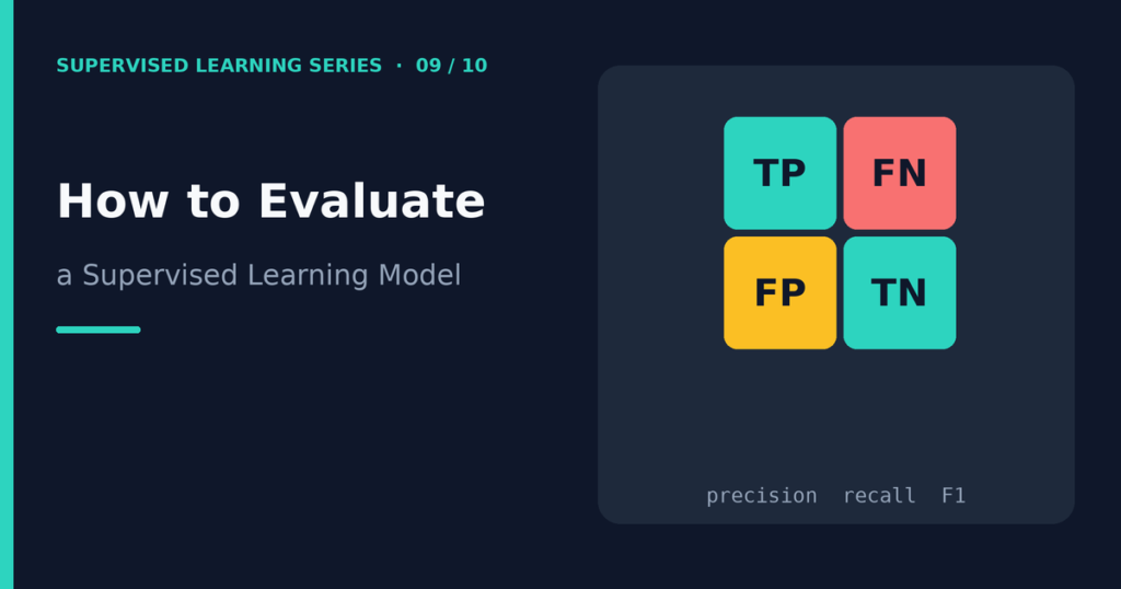
Most classification metrics come from a confusion matrix, a table that counts how often the model’s predictions match the truth. For a binary problem, we call one class “positive” (usually the class you want to find) and the other “negative.” The matrix has four cells:

	Predicted positive	Predicted negative
Actually positive	True positives (TP)	False negatives (FN)
Actually negative	False positives (FP)	True negatives (TN)

• True positive: the model said positive, and it was right.
• True negative: the model said negative, and it was right.
• False positive: the model said positive, but the example was negative (a false alarm).
• False negative: the model said negative, but the example was positive (a miss).

Note that scikit-learn’s confusion_matrix function puts the true classes in rows and the predicted classes in columns, and it orders them by class label. With labels 0 and 1, the layout is [[TN, FP], [FN, TP]]. Always check which class counts as positive in your project.

Classification metrics

Accuracy

Accuracy is the share of all predictions that are correct:

Accuracy = (TP + TN) / (TP + TN + FP + FN)

It is simple and easy to explain, but it can mislead you when classes are imbalanced.

Precision

Precision asks: “Of everything the model called positive, how much really was positive?”

Precision = TP / (TP + FP)

High precision means few false alarms. Precision matters when false positives are costly, such as flagging a legitimate email as spam.

Recall

Recall (also called sensitivity or the true positive rate) asks: “Of all the truly positive examples, how many did the model find?”

Recall = TP / (TP + FN)

High recall means few misses. Recall matters when false negatives are costly, such as missing a fraudulent transaction or a patient who needs follow-up tests.

F1-score

Precision and recall often pull in opposite directions. The F1-score combines them using the harmonic mean:

F1 = 2 × (Precision × Recall) / (Precision + Recall)

The harmonic mean punishes imbalance between the two. A model with precision 1.0 and recall 0.1 gets an F1 of only about 0.18. Use F1 when you care about both kinds of error and want one number.

Specificity

Specificity is the recall of the negative class: TN / (TN + FP). It tells you how well the model recognizes negatives.

Class imbalance

Class imbalance means one class is much rarer than the other. Fraud, rare diseases, and equipment failures all produce imbalanced data. In these cases, accuracy can look wonderful while the model is useless.

Consider 100 transactions, of which 5 are fraud. A “model” that always predicts “not fraud” gets 95 out of 100 right. Its accuracy is 95%, yet it finds none of the fraud. Its recall for fraud is zero. I verified this with a short script: always predicting the majority class gives an accuracy of 0.95 and a recall of 0.0 on that example.

For imbalanced problems, look at precision, recall, and F1 for the rare class, and examine the confusion matrix directly. The precision-recall curve and its area (PR-AUC) are often more informative than ROC-AUC when positives are rare. Some practitioners also use class weights during training or resampling. If you resample, do it only on the training data, never on the test data.

ROC curve and ROC-AUC

Many classifiers output a probability or a score, and you convert it to a class using a threshold. The ROC curve (receiver operating characteristic) shows how the model performs across all possible thresholds. It plots the true positive rate (recall) against the false positive rate (FP / (FP + TN)).

The AUC (area under the curve) compresses the curve into one number between 0 and 1. A value of 0.5 means the model ranks examples no better than chance. A value of 1.0 means it ranks every positive example above every negative one. A useful reading is this: ROC-AUC equals the probability that the model gives a randomly chosen positive example a higher score than a randomly chosen negative example.

ROC-AUC does not depend on a threshold, which makes it handy for comparing models. It does not tell you which threshold to use, and it can look overly optimistic on heavily imbalanced data.

Threshold selection

The default threshold of 0.5 is only a convention. Moving it changes the balance between precision and recall:

• Lower threshold: the model predicts “positive” more often. Recall rises, and precision usually falls.
• Higher threshold: the model predicts “positive” less often. Precision usually rises, and recall falls.

Choose the threshold by the real cost of mistakes. If a missed case is ten times worse than a false alarm, pick a threshold that favors recall. Select it on a validation set or with cross-validation, not on the final test set. The article on logistic regression explains how probabilities and thresholds fit together.

Regression metrics

Regression models predict numbers, so we measure how far the predictions land from the truth. Let yᵢ be the true value, ŷᵢ the prediction, and n the number of examples.

MAE: mean absolute error

MAE = (1/n) × Σ |yᵢ − ŷᵢ|

MAE is the average size of the errors, in the same units as the target. It is easy to explain: “On average, we miss by 40 units.” It treats all errors equally.

MSE: mean squared error

MSE = (1/n) × Σ (yᵢ − ŷᵢ)²

MSE squares the errors, so large errors count much more than small ones. Its units are the squared target units, which makes it hard to interpret directly.

RMSE: root mean squared error

RMSE = √MSE

RMSE returns to the target’s units while still punishing large errors. RMSE is always at least as large as MAE. A big gap between the two signals that a few large errors dominate.

R-squared

R² = 1 − (sum of squared residuals) / (total variation of y around its mean)

R² compares your model with a simple baseline that always predicts the average target. A score of 1 means perfect predictions. A score of 0 means no better than the baseline. It can be negative on test data when the model does worse than the baseline. R² is unitless, which makes it good for a quick check, but it hides the actual size of the errors. Pair it with MAE or RMSE.

How to choose a metric

Situation	Useful metrics	Reason
Balanced classes, equal error costs	Accuracy, F1	Simple and adequate
Missing a positive is costly	Recall, F2 or recall at a set precision	You want to catch as many positives as possible
False alarms are costly	Precision	You want predictions you can trust
Rare positive class	Precision, recall, F1, PR-AUC	Accuracy hides failure on the rare class
Comparing models across thresholds	ROC-AUC, PR-AUC	Threshold-independent ranking quality
Regression, errors matter linearly	MAE	Direct and robust to outliers
Regression, large errors are very bad	RMSE	Penalizes big misses
Explaining overall fit	R² plus an error metric	Shows relative and absolute performance

Always connect the metric to the real decision. Ask: “What happens when the model is wrong, and which wrong answer hurts more?”

Python example

This script trains a logistic regression model, prints the confusion matrix and metrics at two thresholds, and then evaluates a linear regression model on a different dataset. It also repeats the “always predict the majority class” check.

import numpy as np
from sklearn.datasets import load_breast_cancer, load_diabetes
from sklearn.model_selection import train_test_split
from sklearn.pipeline import make_pipeline
from sklearn.preprocessing import StandardScaler
from sklearn.linear_model import LogisticRegression, LinearRegression
from sklearn.metrics import (confusion_matrix, precision_score, recall_score, f1_score,
                             roc_auc_score, accuracy_score, mean_absolute_error,
                             mean_squared_error, r2_score)

# Classification: class 1 (benign) is treated as the positive class
X, y = load_breast_cancer(return_X_y=True)
X_train, X_test, y_train, y_test = train_test_split(
    X, y, test_size=0.2, stratify=y, random_state=42)
clf = make_pipeline(StandardScaler(), LogisticRegression(max_iter=1000)).fit(X_train, y_train)
proba = clf.predict_proba(X_test)[:, 1]

for t in [0.5, 0.9]:
    pred = (proba >= t).astype(int)
    print("threshold", t)
    print(confusion_matrix(y_test, pred))
    print(" acc", round(accuracy_score(y_test, pred), 3),
          "prec", round(precision_score(y_test, pred), 3),
          "rec", round(recall_score(y_test, pred), 3),
          "f1", round(f1_score(y_test, pred), 3))
print("ROC-AUC", round(roc_auc_score(y_test, proba), 3))

# Regression
Xd, yd = load_diabetes(return_X_y=True)
Xtr, Xte, ytr, yte = train_test_split(Xd, yd, test_size=0.2, random_state=42)
p = LinearRegression().fit(Xtr, ytr).predict(Xte)
print("MAE", round(mean_absolute_error(yte, p), 1),
      "MSE", round(mean_squared_error(yte, p), 1),
      "RMSE", round(float(np.sqrt(mean_squared_error(yte, p))), 1),
      "R2", round(r2_score(yte, p), 3))

# The accuracy trap on imbalanced data
yi = np.array([0] * 95 + [1] * 5)
print("always-predict-0 accuracy:", accuracy_score(yi, np.zeros(100, dtype=int)),
      "recall:", recall_score(yi, np.zeros(100, dtype=int)))

When I ran this with Python 3.12 and scikit-learn 1.8.0, the output was:

threshold 0.5
[[41  1]
 [ 1 71]]
 acc 0.982 prec 0.986 rec 0.986 f1 0.986
threshold 0.9
[[41  1]
 [11 61]]
 acc 0.895 prec 0.984 rec 0.847 f1 0.91
ROC-AUC 0.995
MAE 42.8 MSE 2900.2 RMSE 53.9 R2 0.453
always-predict-0 accuracy: 0.95 recall: 0.0

Here is how to read it:

• At threshold 0.5, the model makes just two mistakes in 114 test samples: one false positive and one false negative. Precision and recall are both about 0.986.
• Raising the threshold to 0.9 makes the model more cautious about predicting the positive class (benign). The false negatives jump from 1 to 11, so recall falls from 0.986 to 0.847, while precision stays about the same at 0.984. Accuracy drops to 0.895. This is the precision-recall trade-off in action.
• The ROC-AUC of 0.995 does not change with the threshold, because it summarizes performance across all of them.
• For the regression model, the RMSE of 53.9 is larger than the MAE of 42.8, which tells you that some larger errors push the RMSE up. An R² of 0.453 means the model explains less than half of the variation in this target, which is a modest fit for a plain linear model on this dataset.
• The last line confirms the accuracy trap: 95% accuracy with zero recall.

Your numbers can differ slightly with other versions or seeds. Scores from a single split can also be noisy, so use cross-validation when you compare models closely.

Frequently asked questions

What is the best metric for evaluating a classification model?

No single metric is best. Accuracy works for balanced classes with equal error costs. For imbalanced data or unequal costs, use precision, recall, F1, or PR-AUC. Choose based on which mistakes matter most.

What is the difference between precision and recall?

Precision measures how many predicted positives were truly positive. Recall measures how many true positives the model found. Precision punishes false alarms, and recall punishes misses.

What is a good ROC-AUC score?

A score of 0.5 equals random ranking, and 1.0 equals perfect ranking. Whether a value in between is “good” depends on the problem and on how simple baselines perform. Compare against a baseline model on the same data.

Should I use MAE or RMSE?

Use MAE when you want an easy-to-explain average error and all errors matter equally. Use RMSE when large errors are especially harmful. Reporting both often tells a richer story.

Can R-squared be negative?

Yes. On test data, R² turns negative when the model predicts worse than a constant guess equal to the average training target. It signals a poor or overfit model.

Why is my accuracy high but my model still bad?

Class imbalance is the usual reason. If one class dominates, a model can score high accuracy by predicting that class every time. Check the confusion matrix, precision, and recall for the rare class.

Conclusion

Good evaluation starts with the right question: what kind of mistake matters most? Classification metrics come from the confusion matrix, and regression metrics measure the size of the errors. Class imbalance can make accuracy meaningless, and the decision threshold lets you trade precision against recall. Measure on unseen data, choose metrics in advance, and look beyond a single number.

You now have all the pieces for a complete project. Put them to work in Build Your First Supervised Machine Learning Model with Python.

This article is for educational and informational purposes only. Examples and code are provided to help readers understand model evaluation and may require adaptation for specific projects.

Related guides

Good evaluation starts with a sound data split. Read Training Data vs Testing Data and follow the full workflow in Build Your First Supervised Machine Learning Model with Python.

References and further reading

• Metrics and scoring: quantifying the quality of predictions (scikit-learn user guide) for the definitions and functions used above.
• confusion_matrix documentation (scikit-learn) for the row and column layout.