
Policy Gradient Methods Explained: Learning Policies Directly
Learn policy gradient methods: the policy gradient theorem, REINFORCE, log-probabilities and a tested PyTorch CartPole agent that learns a policy directly.
 Nov 21, 2026Published
22 min readReading time
Everything we have built so far estimates values. Q-learning, SARSA and DQN all learn how good each action is, and then act by picking the best one. That indirect route works well for many problems, but it hides a quiet assumption: that the best behavior can be read off a table of action values by taking a maximum. What if the action is a steering angle or a motor torque, so there is no short list of actions to take a maximum over? What if the best behavior is deliberately random?
Policy gradient methods take a different route. They skip the value estimates and learn the policy itself: a function that maps a state straight to an action or to a probability for each action. The agent improves that function by nudging its parameters toward actions that earned high returns and away from actions that did not. This guide explains why value-based methods can fall short, what a policy and its parameters are, the policy objective, the policy gradient theorem, and the REINFORCE algorithm. Then we build a working REINFORCE agent in PyTorch, train it on CartPole with Gymnasium, and look at the results honestly.
This is the fourth algorithm in our sequence and a deliberate change of direction. Read Deep Q-Networks (DQN) Explained: From Q-Learning to Deep Reinforcement Learning first if you have not, because we compare against it throughout. For the foundations, see What Is Reinforcement Learning? A Complete Guide.
Value-Based Reinforcement Learning and Its Limitations
Value-based reinforcement learning learns a value function, such as Q(s, a), that estimates the expected return of each action. The policy is not learned directly. It is implied: pick the action with the highest value, possibly with some epsilon-greedy randomness added for exploration. Q-learning, SARSA and DQN all work this way.
This approach has real limitations, and each one motivates a policy-based alternative.
- Continuous actions are awkward. Acting means computing the maximum over all actions. With a handful of discrete actions that is trivial. With a continuous action such as a joint torque, the maximum is a separate optimization problem to solve at every single step.
- The policy can change abruptly. The policy is an argmax over values. A tiny change in the estimates can flip which action is best, so the behavior can jump even when the values barely moved. Policy-based methods change behavior smoothly, because the parameters move a little at a time.
- It cannot represent some of the best policies. Value-based methods end up with a deterministic policy, or one that is nearly deterministic. But in some problems the best policy is random. In rock-paper-scissors against an opponent who adapts, the best strategy is to choose each option with equal probability, and any deterministic strategy can be exploited. A policy that outputs probabilities can represent this directly.
- Accurate values are not the goal. A value-based agent spends effort estimating the value of every action, even though all that matters for behavior is which action is best. A policy method optimizes the behavior itself.
What Is a Policy?
A policy, written π, is the agent’s rule for acting. We have used the idea since the first article in the series; here it moves from the background to the center. There are two kinds.
Stochastic policies
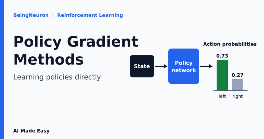
A stochastic policy maps a state to a probability distribution over actions, written π(a | s): the probability of taking action a in state s. The agent samples from this distribution. A CartPole policy might say “in this state, push left with probability 0.73 and right with probability 0.27”. Stochastic policies explore on their own, since every action with nonzero probability gets tried, and they can represent the random strategies described above.
Deterministic policies
A deterministic policy maps a state to exactly one action, written a = μ(s). It is simpler to execute and is what you usually want to deploy after training. Methods that learn deterministic policies directly exist, such as the deterministic policy gradient, but the basic policy gradient algorithm in this article learns a stochastic policy. For continuous actions, a common stochastic choice is a Gaussian: the network outputs a mean (and often a spread), and the agent samples the action from that bell curve.
| Property | Stochastic policy π(a | s) | Deterministic policy a = μ(s) |
|---|---|---|
| Output | A probability for each action (or a distribution over a continuous range) | One action |
| Exploration | Built in, since actions are sampled | Must be added, for example with noise |
| Can express “randomize on purpose” | Yes | No |
| Typical use | Training with basic policy gradients | Deployment, or specialized algorithms |
Learning a Value Function vs Learning a Policy Directly
This is the central shift of the article, so here it is as a picture. The two families both start from a state and end in an action. They differ in what the network outputs, and therefore in what it is trained to get right.
| Aspect | Value-based (for example DQN) | Policy-based (for example REINFORCE) |
|---|---|---|
| What is learned | Action values Q(s, a) | The policy π(a | s) itself |
| How actions are chosen | Argmax over values, plus epsilon-greedy exploration | Sampling from the learned distribution |
| Action spaces | Small discrete sets | Discrete or continuous |
| Stochastic policies | Only through added exploration noise | Natural and learnable |
| Behavior change per update | Can jump when the best action flips | Smooth, as parameters change gradually |
| Data use | Off-policy: old experience can be replayed | On-policy in the basic form: data must come from the current policy |
| Main weakness | Instability, discrete actions only | High variance, sample inefficiency |
Neither family is simply better. Many practical algorithms combine the two, which is where the next article in this series goes.
Policy Parameters and the Policy Network
To learn a policy, we need to write it as a function we can adjust. The standard approach is to use a neural network with weights θ, called the policy parameters, and write the policy as πθ(a | s). Changing θ changes the policy. Learning means finding good values of θ.
For a discrete action space, the network takes the state and outputs one raw score, called a logit, for each action. A softmax turns the logits z into probabilities that are positive and sum to 1:
πθ(a | s) = exp(za) / Σb exp(zb)
Here za is the logit of action a, and the sum runs over all actions b. A larger logit means a larger probability. For example, logits of 1.0 and 0.0 give probabilities 0.731 and 0.269.
The change from the DQN network is small in structure and large in meaning. The Q-network’s outputs were unbounded estimates of return. The policy network’s outputs are scores that become a probability distribution, and nothing in the network estimates a return at all.
The Policy Objective
To improve a policy we need a number that says how good it is. The natural choice is the expected return: the total discounted reward the agent collects, averaged over many episodes of acting with the policy.
A trajectory τ is one complete run: a sequence of states, actions and rewards (s0, a0, r1, s1, a1, …). Its return is the discounted sum of its rewards, R(τ) = r1 + γ r2 + γ2 r3 + …, with the discount factor γ explained in earlier articles. The objective is the average return over trajectories generated by the policy:
| Symbol | Meaning |
|---|---|
| J(θ) | The objective: the expected return of the policy with parameters θ. Higher is better. |
| τ ∼ πθ | A trajectory generated by acting with the policy πθ. |
| R(τ) | The discounted return of that trajectory. |
| E[ … ] | The average over many trajectories. |
| α | The learning rate, the step size of each update. |
| ∇θ J(θ) | The gradient: for each parameter, how much J would change if that parameter increased slightly. |
Note that this is gradient ascent, because we are maximizing a score. Deep learning libraries minimize losses, so the code later minimizes the negative of the objective. Everything now depends on one question: how do we compute ∇θ J(θ)? The return depends on the environment’s dynamics, which the agent does not know, and sampling an action is a random step that does not look differentiable.
The Policy Gradient Theorem
The answer is a neat identity called the log-derivative trick. For any probability p, the gradient satisfies ∇p = p · ∇log p. Apply it to the probability of a whole trajectory, which is a product of three kinds of terms: the starting-state probability, the policy’s action probabilities πθ(at | st), and the environment’s transition probabilities. When we take the logarithm, the product becomes a sum. Only the policy terms depend on θ, so the starting-state and environment terms disappear from the gradient. The result is:
This is remarkable for two reasons. First, it does not require a model of the environment: the gradient can be estimated purely from sampled experience. Second, it has a simple reading. For each action taken, the term ∇log πθ(at | st) points in the direction in parameter space that makes that action more likely, and it is scaled by Gt, how good the outcome was. So the update says: make actions that were followed by high returns more probable, and actions followed by low returns less probable.
Two details are worth knowing. In the formula above I used the return from step t onward, Gt (“reward-to-go”), rather than the whole-episode return R(τ). This is allowed because an action cannot affect rewards that came before it, and it reduces noise without changing the expected gradient. The more general result, the policy gradient theorem (Sutton et al., 2000), states that the gradient can be written with the action-value function: ∇J(θ) = E[∇log πθ(a | s) · Qπ(s, a)]. REINFORCE replaces the true Qπ(s, a) with the sampled return Gt, which has the same expected value.
The log-probability and its gradient
The log-probability is the key building block, so it is worth seeing concretely. For a softmax policy, the gradient of log π(a) with respect to the logits has a clean form: a vector with 1 at the chosen action, minus the vector of probabilities. In symbols, ∂ log π(a) / ∂zb = 1[b = a] − π(b). So if the policy gave the chosen action probability 0.73, its logit is pushed up by 0.27 per unit of weight, and every other logit is pushed down by that action’s share. An action that was already very likely produces a small push; an unlikely one produces a large push. A framework like PyTorch computes this automatically through backpropagation once you have log_prob, which is why the code is short.
A Numerical Example: How One Update Changes the Policy
Take a policy over two actions with logits z = (1.0, 0.0). The probabilities are π = (0.7311, 0.2689). Suppose the agent samples action 0 and the return that followed is G = +2. Use a step size of 0.1 and, to keep the arithmetic visible, treat the logits themselves as the parameters.
- Gradient of log π(0): 1[b = 0] − π(b) gives (1 − 0.7311, 0 − 0.2689) = (0.2689, −0.2689).
- Scale by the return and step size: 0.1 × 2 × (0.2689, −0.2689) = (0.0538, −0.0538).
- New logits: (1.0538, −0.0538), which give probabilities (0.7517, 0.2483).
Action 0 became more likely, rising from 0.7311 to 0.7517. Now suppose the same action had been followed by a bad return, G = −2. The same steps give logit changes of (−0.0538, +0.0538), new logits (0.9462, 0.0538), and probabilities (0.7094, 0.2906). Action 0 became less likely. The return acts as a signed weight: positive strengthens the action that was taken, negative weakens it.
The REINFORCE Algorithm
REINFORCE, introduced by Ronald Williams in 1992, turns the formula above into an algorithm. It is a Monte Carlo method: it waits until an episode finishes, then uses the actual returns that followed each action. The recipe:
- Initialize the policy network with random parameters θ.
- Run one full episode with the current policy, sampling each action from πθ(a | s), and record every state, action and reward.
- Compute the return Gt for each step, working backward from the end of the episode.
- Compute the loss −Σt log πθ(at | st) · Gt. The minus sign turns gradient ascent into the descent that optimizers perform.
- Take a gradient step to update θ.
- Discard the episode and repeat with a fresh one. The data came from the old policy, so it cannot be reused.
REINFORCE pseudocode
initialize policy network pi(a | s; theta) with random weights

for each episode:
    generate a trajectory s0, a0, r1, s1, a1, r2, ... by sampling a_t from pi(. | s_t; theta)

    for each step t:
        G_t = r_(t+1) + gamma * r_(t+2) + gamma^2 * r_(t+3) + ...     # return from step t

    loss = - sum over t of ( log pi(a_t | s_t; theta) * G_t )
    update theta by gradient descent on loss                          # equals gradient ascent on J
Variance reduction: reward-to-go and baselines
REINFORCE’s weakness is noise. A single episode is one random sample, and the return Gt can vary enormously between episodes, so the gradient estimate is jumpy. Two simple ideas help.
- Reward-to-go (used above) uses only the rewards after step t, since earlier rewards cannot depend on the action taken at t.
- A baseline subtracts a number b(s) from the return: use (Gt − b(st)) in place of Gt. If the baseline depends only on the state, it does not change the expected gradient, but it can cut the variance a lot. Intuitively, it lets the agent ask “was this better than usual?” instead of “was this positive?”. When all returns are positive, as in CartPole, every action would otherwise be pushed up, just by different amounts.
The code below uses a simple practical version: it standardizes the returns within each episode (subtract their mean, divide by their standard deviation). This is a common trick rather than a state-dependent baseline, so strictly speaking it slightly changes the gradient, but it makes training far steadier in practice. A learned baseline, the value function, is the idea behind the actor-critic methods in the next article.
Implementing REINFORCE in PyTorch
We train on CartPole-v1, the same environment as in the DQN article, so you can compare the two approaches directly. The agent pushes a cart left or right to keep a pole upright, earns +1 per step, and the maximum return is 500 because episodes are cut off at 500 steps.
Installation. Run pip install torch gymnasium numpy. Copy the stages below, in order, into one file named reinforce_cartpole.py. I ran this exact script on a single CPU core with Python 3.12.3, PyTorch 2.15.0, Gymnasium 1.4.0 and NumPy 2.5.4. Training takes a few minutes.
Stage 1: Imports and hyperparameters
import random

import gymnasium as gym
import numpy as np
import torch
import torch.nn as nn
from torch.distributions import Categorical

SEED = 0
ENV_NAME = "CartPole-v1"

GAMMA = 0.99
LEARNING_RATE = 3e-3
EPISODES = 800
HIDDEN = 128
The constants set the discount factor, the learning rate, the number of training episodes (each one is a single update) and the hidden layer size. Categorical is PyTorch’s distribution over a fixed set of choices, which handles softmax, sampling and log-probabilities for us.
Stage 2: The policy network
class PolicyNetwork(nn.Module):
    """State in, one score (logit) per action out."""

    def __init__(self, state_dim, n_actions, hidden=HIDDEN):
        super().__init__()
        self.net = nn.Sequential(
            nn.Linear(state_dim, hidden), nn.ReLU(),
            nn.Linear(hidden, n_actions),
        )

    def forward(self, state):
        return Categorical(logits=self.net(state))       # softmax over the logits
This is Figure 2. A hidden layer of 128 units maps the 4 state numbers to 2 logits. Instead of returning raw numbers, forward wraps them in a Categorical distribution, which applies the softmax internally. Calling the network on a state therefore gives back a probability distribution over actions that we can sample from.
Stage 3: Running an episode
def run_episode(env, policy):
    state, _ = env.reset()
    log_probs, rewards = [], []
    done = False
    while not done:
        dist = policy(torch.as_tensor(state, dtype=torch.float32))
        action = dist.sample()                            # sample from pi(a|s)
        log_probs.append(dist.log_prob(action))           # log pi(a|s), kept for the gradient
        state, reward, terminated, truncated, _ = env.step(action.item())
        rewards.append(reward)
        done = terminated or truncated
    return log_probs, rewards
The agent plays one full episode. At each step it asks the policy for a distribution, samples an action, and stores dist.log_prob(action), the log-probability of the action it just took. This stored value is still connected to the network’s computation graph, which is what lets PyTorch compute ∇log π later. The environment returns the next state and reward, and the loop stops when the episode ends or is truncated at 500 steps.
Stage 4: Computing returns
def compute_returns(rewards, gamma=GAMMA):
    """Reward-to-go: G_t = r_t + gamma * r_(t+1) + gamma^2 * r_(t+2) + ..."""
    returns, running = [], 0.0
    for r in reversed(rewards):
        running = r + gamma * running
        returns.append(running)
    returns.reverse()
    return torch.tensor(returns, dtype=torch.float32)
This computes Gt for every step by walking backward through the rewards. Starting from the end, each return is the current reward plus γ times the return of the following step. Going backward makes this one pass instead of a nested loop. The list is then reversed so that position t holds Gt.
Stage 5: Training
def train(seed=SEED, episodes=EPISODES, lr=LEARNING_RATE, log=True):
    random.seed(seed)
    np.random.seed(seed)
    torch.manual_seed(seed)

    env = gym.make(ENV_NAME)
    env.reset(seed=seed)
    policy = PolicyNetwork(env.observation_space.shape[0], env.action_space.n)
    optimizer = torch.optim.Adam(policy.parameters(), lr=lr)
    episode_returns = []

    for episode in range(1, episodes + 1):
        log_probs, rewards = run_episode(env, policy)
        returns = compute_returns(rewards)
        returns = (returns - returns.mean()) / (returns.std() + 1e-8)   # variance reduction

        loss = -(torch.stack(log_probs) * returns).sum()  # minus sign: gradient ASCENT on J
        optimizer.zero_grad()
        loss.backward()
        optimizer.step()

        episode_returns.append(sum(rewards))
        if log and episode % 50 == 0:
            print(f"episode {episode:4d} | avg return (last 50) {np.mean(episode_returns[-50:]):6.1f}")

    env.close()
    return policy, episode_returns
Each iteration is one episode and one update. After the episode, the code computes the returns and standardizes them (the variance-reduction step). The loss line is the heart of the algorithm: it multiplies each stored log-probability by its return, sums them, and negates the result. Minimizing this negative number is the same as maximizing Σ log π · G. Then backward() computes the gradient through all the stored log-probabilities and the optimizer takes a step. The episode’s data is then simply dropped, because the next iteration starts a fresh episode with the updated policy.
Stage 6: Evaluation
def evaluate(policy, episodes=20, seed=1234, greedy=True):
    env = gym.make(ENV_NAME)
    scores = []
    for i in range(episodes):
        state, _ = env.reset(seed=seed + i)
        done, total = False, 0.0
        while not done:
            with torch.no_grad():
                dist = policy(torch.as_tensor(state, dtype=torch.float32))
                action = dist.probs.argmax() if greedy else dist.sample()
            state, reward, terminated, truncated, _ = env.step(action.item())
            total += reward
            done = terminated or truncated
        scores.append(total)
    env.close()
    return scores


if __name__ == "__main__":
    model, _ = train()
    greedy_scores = evaluate(model, greedy=True)
    sampled_scores = evaluate(model, greedy=False)
    print(f"\nGreedy  evaluation (20 episodes): mean = {np.mean(greedy_scores):.1f}, "
          f"min = {np.min(greedy_scores):.0f}, max = {np.max(greedy_scores):.0f}")
    print(f"Sampled evaluation (20 episodes): mean = {np.mean(sampled_scores):.1f}, "
          f"min = {np.min(sampled_scores):.0f}, max = {np.max(sampled_scores):.0f}")
Evaluation uses fresh start conditions and no learning, and it measures the policy in two ways. Greedy mode always takes the most probable action, which turns the stochastic policy into a deterministic one. Sampled mode keeps sampling from the probabilities, exactly as during training. Comparing the two is instructive, as the results show. Running the script with seed 0 produced:
episode   50 | avg return (last 50)   19.6
episode  100 | avg return (last 50)   25.1
episode  150 | avg return (last 50)   83.2
episode  200 | avg return (last 50)  256.4
episode  250 | avg return (last 50)  233.6
episode  300 | avg return (last 50)  341.7
episode  350 | avg return (last 50)  450.7
episode  400 | avg return (last 50)  471.2
episode  450 | avg return (last 50)  409.2
episode  500 | avg return (last 50)  475.1
episode  550 | avg return (last 50)  413.2
episode  600 | avg return (last 50)  495.8
episode  650 | avg return (last 50)  466.7
episode  700 | avg return (last 50)  494.8
episode  750 | avg return (last 50)  500.0
episode  800 | avg return (last 50)  491.0

Greedy  evaluation (20 episodes): mean = 500.0, min = 500, max = 500
Sampled evaluation (20 episodes): mean = 398.9, min = 11, max = 500Reading the Results Honestly
- It learned. The average return climbed from about 20 to near the maximum of 500, and the greedy policy balanced the pole for all 500 steps in all 20 evaluation episodes on seed 0.
- Seeds. I ran seeds 0 to 4 with the same settings. The greedy evaluation means were 500.0, 500.0, 500.0, 500.0 and 495.9. The sampled evaluation means were 398.9, 500.0, 500.0, 500.0 and 388.6. So every seed learned a strong greedy policy in this test.
- Greedy and sampled differ. On seeds 0 and 4 the sampled policy had occasional disastrous episodes (the worst were 11 and 107 steps), even though the greedy version was nearly perfect. The learned policy is still stochastic, so it sometimes samples an unlucky action in a delicate situation. This is a real property of stochastic policies: you often deploy the greedy version.
- The curve is noisy. Even late in training the average moves between about 410 and 500. That is the variance of REINFORCE showing through.
- Hyperparameters matter. I tried two learning rates on seed 0: 1e-2 reached a greedy mean of 481.1 and a final-100-episode average of 163.3, while 3e-3 reached 500.0 and 495.5. I chose 3e-3 after seeing seed 0, so seed 0 is not an unbiased test, and seeds 1 to 4 are the fairer check. A third setting (1e-3) did not finish in my testing window, so I do not report it.
Five seeds is a small sample, so read these as an illustration, not a benchmark. Your results will differ with other library versions and hardware, because random number streams are not identical across them. Also note that this comparison is not “REINFORCE beats DQN”: the two articles use different hyperparameters, step budgets and update schedules, so the numbers are not a fair head-to-head. CartPole is also a very easy task.
Advantages of Policy Gradient Methods
- Continuous and large action spaces. The policy can output a distribution over actions, so no maximum over actions is needed.
- Stochastic policies. They can represent behavior that must be random, and they explore naturally.
- Smooth improvement. Small parameter changes cause small changes in behavior, which avoids the abrupt flips of argmax policies.
- Direct optimization. The method optimizes the quantity we actually care about, the expected return.
- Foundation for modern algorithms. Actor-critic methods and PPO, covered next, are built on this gradient.
Limitations of Policy Gradient Methods
- High variance. Gradients estimated from single episodes are noisy, which slows and destabilizes learning.
- Sample inefficiency. Basic policy gradients are on-policy, so each episode is used once and discarded.
- Local optima. Gradient ascent can settle on a good but not best policy.
- Waiting for episodes to end. REINFORCE is a Monte Carlo method, so it cannot learn within an episode and is awkward for very long or endless tasks.
- Credit assignment. Every action in an episode shares credit for the total outcome, so it can be hard to tell which action mattered.
- Sensitivity to the learning rate. As the runs above show, too large a step can hurt performance.
- A discounting subtlety. For the discounted objective, the exact gradient weights step t by γt. Most practical implementations, including the code here, leave that factor out, which is a widely used approximation.
Value-Based vs Policy-Based Reinforcement Learning: When to Choose Which
Choose value-based methods like DQN when the actions are few and discrete and you want to reuse past experience for sample efficiency. Choose policy-based methods when the action space is continuous or large, when a stochastic policy is needed, or when you want smooth, stable changes in behavior. In practice the best systems usually combine both, learning a policy and a value function together, which is the subject of the next article.
Applications of Policy Gradient Methods
- Robotics and continuous control. Policy-based methods are a standard choice in research on controlling robot joints and simulated locomotion, where actions are continuous.
- Games. AlphaGo refined its policy network with policy-gradient reinforcement learning from self-play, after first training it on human games.
- Language models. Reinforcement learning from human feedback is commonly implemented with policy-optimization algorithms in the policy gradient family, notably PPO.
- Research and teaching. REINFORCE is the standard first policy-gradient algorithm because its logic is so transparent.
For a wider look at where reinforcement learning is used, see Applications of Reinforcement Learning: 10 Real-World Examples.
Frequently Asked Questions
What are policy gradient methods?
They are reinforcement learning algorithms that learn the policy directly. They adjust the policy’s parameters in the direction that increases expected return, using the gradient of the policy objective.
What is the policy gradient theorem?
It says the gradient of the expected return can be written as an expectation of ∇log π(a | s) multiplied by the value of the action. It lets us estimate the gradient from sampled experience without knowing the environment’s dynamics.
What is the REINFORCE algorithm?
REINFORCE is the basic Monte Carlo policy gradient method. It runs a full episode, computes the return after each action, and increases the probability of actions in proportion to those returns.
Why take the logarithm of the probability?
The log-derivative trick, ∇p = p · ∇log p, lets us turn the gradient of an expectation into an expectation we can estimate by sampling. It also removes the environment’s unknown dynamics from the gradient.
What is the difference between value-based and policy-based reinforcement learning?
Value-based methods learn the value of actions and pick the best one. Policy-based methods learn the policy itself, which makes continuous actions and stochastic behavior natural.
Why do policy gradient methods have high variance?
The gradient is estimated from sampled episodes whose returns vary a lot. Reward-to-go, baselines and actor-critic methods are the standard remedies.
Conclusion and Next Steps
Policy gradient methods learn the policy directly. The central result is simple to say: increase the probability of actions that were followed by high returns, and decrease it for those followed by low returns. The log-derivative trick makes that computable from samples, REINFORCE turns it into an algorithm, and PyTorch’s log-probabilities make it a handful of lines. You have seen it work on CartPole, and you have seen its main weakness, noise.
To practice, try removing the return standardization in the code and watch how learning changes, compare learning rates on several seeds, or swap in a different Gymnasium environment with discrete actions. To review the earlier algorithms, see Deep Q-Networks (DQN) Explained and Q Learning Update Rule Explained: Formula, Algorithm & Python Example, and for the big picture, What Is Reinforcement Learning? A Complete Guide.
The natural next step is to reduce the variance by learning a value function alongside the policy. That combination, the actor-critic architecture, and the algorithm PPO that builds on it, are the subject of the next article in this series, Actor-Critic and PPO Explained: Advanced Deep Reinforcement Learning Algorithms.