Decision Trees in Machine Learning: How They Work

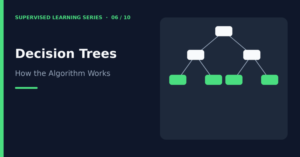
The decision tree algorithm is a supervised learning method that makes predictions by asking a series of simple questions about the features, such as “Is the petal length below 2.45 cm?” Each answer sends an example down one branch of a tree until it reaches a final box, called a leaf, that holds the prediction. A decision tree can classify categories or predict numbers, and people like it because you can read the finished model like a flowchart.

This guide explains how decision trees work. You will learn the parts of a tree, how recursive splitting chooses questions, how Gini impurity, entropy, and information gain measure a good split, and how stopping rules and pruning control overfitting. A Python example with real output closes the article. For the broader context, see What Is Supervised Learning?

The parts of a decision tree

A decision tree looks like an upside-down tree, with the first question at the top. Four terms describe its parts:

• Root node: the first question, at the top. It sees the entire training set.
• Internal node (decision node): any question below the root. Each one splits its examples into two or more groups.
• Branch: the path that an answer takes, for example “yes” or “no.”
• Leaf node: an endpoint with no further questions. A leaf holds the prediction, which is a class label for classification or a number for regression.

To predict, you start at the root, answer each question using the example’s features, follow the matching branch, and repeat until you land on a leaf. The leaf’s value becomes the prediction. Because every step is a plain question, you can explain any individual prediction by listing the path.

How a tree learns: recursive splitting

The algorithm builds the tree from the top down using a process called recursive splitting. In simple terms:

1. Start with all training examples in the root node.
2. For every feature, and every possible cutoff value, try splitting the examples into two groups.
3. Score each candidate split using an impurity measure (explained next), and pick the one that separates the classes best.
4. Apply the same procedure again to each of the two new groups, using only the examples in that group.
5. Stop when a stopping rule applies, and turn the node into a leaf.

The word “recursive” means the algorithm repeats the same steps on smaller and smaller subsets. The method is also greedy: at every node it picks the split that looks best right now, without planning ahead. That is fast, but it does not guarantee the best possible tree overall.

Scikit-learn uses an optimized version of the CART algorithm (Classification and Regression Trees), which builds binary trees. Older algorithms such as ID3 and C4.5 use entropy, and they can create more than two branches for categorical features.

Gini impurity, entropy, and information gain

A good split produces groups that are as pure as possible, meaning each group mostly holds a single class. Impurity measures put a number on this.

Gini impurity

Gini impurity measures the chance of labeling a random example wrongly if you label it by sampling from the node’s class mix. For a node where pₖ is the share of class k:

Gini = 1 − Σ pₖ²

A node that holds only one class has Gini = 0 (perfectly pure). In a two-class problem, a 50/50 mix gives the maximum value, 0.5. Lower is better. Scikit-learn uses Gini by default.

Entropy

Entropy comes from information theory and measures disorder:

Entropy = − Σ pₖ × log₂(pₖ)

A pure node has entropy 0. A 50/50 two-class node has entropy 1. Like Gini, lower is better.

Information gain

Information gain is the drop in impurity that a split produces. You compute the parent node’s impurity, subtract the weighted average impurity of the child nodes (weighted by how many examples each child holds), and the difference is the gain:

Information gain = impurity(parent) − Σ (nᶜʰⁱˡᵈ / nᵖᵃʳᵉⁿᵗ) × impurity(child)

The algorithm picks the split with the highest gain. The term “information gain” usually refers to entropy, but the same pattern works with Gini, where some people call the result “Gini gain.” In practice, Gini and entropy usually choose the same or very similar splits, and Gini is slightly cheaper to compute. Tuning the depth of the tree usually matters far more than choosing between the two.

A worked numeric example

Suppose a node holds 10 customers: 6 bought a product and 4 did not. A candidate question, “Is the customer under 30?”, sends 6 customers left and 4 right. The left group has 5 buyers and 1 non-buyer. The right group has 1 buyer and 3 non-buyers.

Node	Buyers / non-buyers	Gini	Entropy
Parent	6 / 4	0.480	0.971
Left child (6 customers)	5 / 1	0.278	0.650
Right child (4 customers)	1 / 3	0.375	0.811

The weighted Gini of the children is 0.6 × 0.278 + 0.4 × 0.375 ≈ 0.317, so the Gini gain is 0.480 − 0.317 ≈ 0.163. The weighted entropy is 0.6 × 0.650 + 0.4 × 0.811 ≈ 0.715, so the information gain is 0.971 − 0.715 ≈ 0.256. The algorithm would compute the same quantities for every other candidate question and choose the question with the largest gain.

Stopping criteria

If a tree keeps splitting until every leaf is perfectly pure, it memorizes the training data. Stopping criteria prevent this by telling the algorithm when to stop. Common rules include:

• Maximum depth (max_depth): limit how many levels the tree can have.
• Minimum samples to split (min_samples_split): do not split a node that has too few examples.
• Minimum samples per leaf (min_samples_leaf): require each leaf to contain at least a certain number of examples.
• Minimum impurity decrease (min_impurity_decrease): refuse splits that improve purity by too little.
• Maximum leaf nodes (max_leaf_nodes): cap the total number of leaves.
• Pure node: stop when every example in a node has the same label.

Limiting growth while the tree is built is called pre-pruning or early stopping.

Pruning and overfitting

Decision trees overfit easily. An unrestricted tree can carve out tiny regions for individual noisy examples, so it scores perfectly on training data but worse on new data. The article Overfitting vs Underfitting in Machine Learning explains this problem in general. For trees, you have two control strategies:

• Pre-pruning: set the stopping rules above before training.
• Post-pruning: grow a large tree first, then remove branches that add little value. Scikit-learn supports minimal cost-complexity pruning through the ccp_alpha parameter. A higher ccp_alpha removes more branches and gives a smaller tree.

Choose the settings with cross-validation or a validation set, not with the test set. See Training Data vs Testing Data for how to keep that evaluation honest.

Regression trees

Decision trees also predict numbers. A regression tree splits the data in the same recursive way, but it measures split quality with an error measure such as mean squared error, not with Gini or entropy. Each leaf predicts the average target value of the training examples that landed in it. This produces a predicted curve that looks like a staircase. The difference between the two task types is described in Classification vs Regression in Machine Learning.

Python example

The example below trains two trees on the iris dataset, which has 150 flowers from three species and four measurements for each. The first tree has no restrictions. The second tree uses max_depth=3 and min_samples_leaf=3. The code prints the tree as readable text.

from sklearn.datasets import load_iris
from sklearn.model_selection import train_test_split
from sklearn.tree import DecisionTreeClassifier, export_text

iris = load_iris()
X_train, X_test, y_train, y_test = train_test_split(
    iris.data, iris.target, test_size=0.2, stratify=iris.target, random_state=42)

full = DecisionTreeClassifier(random_state=42).fit(X_train, y_train)
small = DecisionTreeClassifier(max_depth=3, min_samples_leaf=3, random_state=42).fit(X_train, y_train)

for name, m in [("unrestricted", full), ("max_depth=3", small)]:
    print(name, "depth", m.get_depth(), "leaves", m.get_n_leaves(),
          "train acc", round(m.score(X_train, y_train), 3),
          "test acc", round(m.score(X_test, y_test), 3))

print(export_text(small, feature_names=iris.feature_names))

When I ran this with Python 3.12 and scikit-learn 1.8.0, the output was:

unrestricted depth 5 leaves 8 train acc 1.0 test acc 0.933
max_depth=3 depth 3 leaves 5 train acc 0.983 test acc 0.967
|--- petal length (cm) <= 2.45
|   |--- class: 0
|--- petal length (cm) >  2.45
|   |--- petal width (cm) <= 1.65
|   |   |--- petal length (cm) <= 4.95
|   |   |   |--- class: 1
|   |   |--- petal length (cm) >  4.95
|   |   |   |--- class: 2
|   |--- petal width (cm) >  1.65
|   |   |--- petal length (cm) <= 4.85
|   |   |   |--- class: 2
|   |   |--- petal length (cm) >  4.85
|   |   |   |--- class: 2

Read the text output from the top. The root question is “Is the petal length at most 2.45 cm?” If yes, the flower is class 0 (setosa). If no, the tree asks about petal width, and then petal length again, until it reaches a class.

The comparison shows overfitting in action. The unrestricted tree fits the training data perfectly (accuracy 1.0) but scores 0.933 on the test set. The restricted tree gives up a little training accuracy (0.983) and scores 0.967 on the test set. The test set here holds only 30 flowers, so one flower changes the accuracy by about 0.033. Treat the difference as an illustration, not as proof that restricted trees always win. Use cross-validation for real decisions.

You may also notice that the last two leaves both predict class 2. Splits like this still reduce impurity inside the node, even though the final label does not change. That is a normal property of impurity-based splitting.

Advantages and limitations

Advantages

• Easy to explain. You can show the tree to a non-technical person.
• Little preparation. Trees do not need feature scaling, and they work with numeric thresholds directly.
• Handles non-linear patterns. Trees capture interactions between features without manual engineering.
• Works for both tasks. One method covers classification and regression.

Limitations

• Overfits without limits. Deep trees memorize noise.
• Unstable. A small change in the training data can produce a completely different tree.
• Axis-aligned splits. Each question uses one feature, so diagonal boundaries need many splits.
• Cannot extrapolate. A regression tree never predicts outside the range of target values it saw in training.
• Greedy construction. The tree may miss better overall structures.

The instability problem is exactly what ensembles fix. Read Random Forest vs Decision Tree: Key Differences to see how combining many trees improves results.

Frequently asked questions

What is the difference between Gini impurity and entropy?

Both measure how mixed the classes are in a node. Entropy uses logarithms and ranges from 0 to 1 for two classes, while Gini uses squares and ranges from 0 to 0.5. They usually pick very similar splits, and Gini is slightly faster to compute.

How does a decision tree choose where to split?

It tests candidate questions on every feature and picks the one that gives the largest impurity reduction, which is the highest information gain. It then repeats the process inside each new group.

Do decision trees need feature scaling?

No. A split compares a feature with a threshold, so the scale of the feature does not change which examples fall on each side.

How do I stop a decision tree from overfitting?

Limit the tree with max_depth, min_samples_leaf, or min_samples_split, or apply cost-complexity pruning with ccp_alpha. Tune these settings using cross-validation. You can also switch to a random forest.

Can decision trees handle missing values?

It depends on the implementation. Recent scikit-learn versions support missing values in some tree estimators, but you should check the documentation for your version. When in doubt, fill missing values with an imputer inside a pipeline.

Are decision trees good for beginners?

Yes. They are intuitive, they need little preprocessing, and you can inspect the result. They also introduce the central ideas of overfitting and model complexity in a very visible way.

Conclusion

A decision tree learns by repeatedly asking the question that best separates the data. Gini impurity or entropy score each candidate question, information gain picks the winner, and stopping rules or pruning keep the tree from growing too complicated. The result is a model that you can read, explain, and use for classification or regression.

The weakness of a single tree is its instability. The next article, Random Forest vs Decision Tree, shows how many trees together can give more reliable predictions.

This article is for educational and informational purposes only. Examples and code are provided to help readers understand the decision tree algorithm and may require adaptation for specific projects.

Related guides

See how ensembles improve on a single tree in Random Forest vs Decision Tree, and learn how to evaluate the resulting model in How to Evaluate a Supervised Learning Model.

References and further reading

• Decision Trees (scikit-learn user guide) for parameters, CART, and cost-complexity pruning.
• What is a decision tree? (IBM) for another introduction to entropy, information gain, and Gini impurity.