
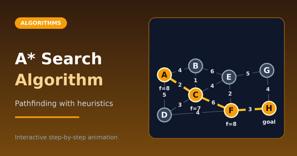
A* Search Algorithm
Learn the A* search algorithm with an interactive pathfinding visualization, step-by-step example, heuristics, pseudocode, JavaScript code, and complexity.
Learn the A* search algorithm with an interactive pathfinding visualization, step-by-step example, heuristics, pseudocode, JavaScript code, and complexity.

Understand the bubble sort algorithm with an interactive visualization, step-by-step example, pseudocode, JavaScript code, and complexity analysis.

Learn Prim’s algorithm for minimum spanning trees with an interactive visualization, step-by-step example, pseudocode, JavaScript code, and complexity.

Learn the insertion sort algorithm with an interactive step-by-step visualization, example, pseudocode, JavaScript code, and time and space complexity.

The Quick Sort algorithm sorts an array by picking a pivot, partitioning the other items around it, and repeating on the smaller parts. Use the visualization below to run it, pause it, step through it, and even step backward. ▶ Play⏮ BackStep ⏭↺ ResetRun to completionShuffle SpeedVery SlowSlowNormalFastVery Fast PivotLast elementFirst elementMiddle elementRandom element Size (5–60) Min Max Generate new array Apply arrayUnsortedP = pivot? = compared⇄ = swapped✓ = final positioni = partition boundaryactive subarray Operation log Recursive calls Complexity (theory): best O(n log n), average O(n log n), worst O(n²). Extra space: O(log n) stack when balanced, O(n) worst case. In-place partitioning, usually not stable. Real behavior depends on pivot choice, input and implementation. The counters above are measured for your array only. Introduction to Quick Sort Quick Sort is a comparison-based sorting algorithm and one of the best-known divide and conquer algorithms. Developers use it because it is simple, sorts in place, and is fast on many real inputs. Its key idea is partitioning: rearrange items so the pivot lands in its final position, with items that belong before it on one side and items that belong after it on the other. Learning Quick Sort is a great way to understand sorting algorithms and recursion. What Is the Quick Sort Algorithm? The Quick Sort algorithm sorts an array by choosing one element, the pivot, and partitioning the rest around it. After partitioning, the pivot never moves again. Quick Sort then sorts the left part and the right part the same way. Take [3, 1, 2]. With pivot 2, the value 1 goes left and 3 stays right, giving [1, 2, 3]. Each step shrinks the problem until pieces are too small to need sorting. How Quick Sort Works Step by Step Choose a pivot. Partition the array around the pivot. Recursively sort the left subarray. Recursively sort the right subarray. Finish when each subarray has zero or one element. The exact moves in step 2 depend on the partition scheme. This page uses the Lomuto scheme for every pivot strategy: the chosen pivot is first swapped to the end of the subarray, then partitioned. Its invariant: while scanning, items from the start up to boundary i hold values less than or equal to the pivot, and items from i up to the scan position hold values greater than the pivot. Because of the “less than or equal” rule, equal values may sit on the left, so do not assume everything on the left is strictly smaller. Understanding the Pivot in Quick Sort The pivot is the reference value for a partition. Pivot choice matters because it decides how even the two parts are. Common strategies: First element: easy, but slow on already sorted input. Last element: also easy and equally weak on sorted input. Middle element: handles sorted and reverse-sorted arrays well. Note that the middle index is not the median value. Random element: makes consistently bad splits unlikely. Median of three (optional): use the median of the first, middle and last values for better balance. Try each strategy in the visualization on a sorted array and compare the comparison counts. Quick Sort Example With a Step-by-Step Walkthrough Array [8, 3, 1, 7, 0, 10, 2], Lomuto partition, last element as pivot. Pivot is 2, boundary i = 0. Scan: 8 and 3 are greater than 2, so nothing moves. 1 is at most 2, so swap it with index 0: [1, 3, 8, 7, 0, 10, 2], i = 1. 7 is greater. 0 is at most 2, so swap with index 1: [1, 0, 8, 7, 3, 10, 2], i = 2. 10 is greater. Place the pivot: swap index 2 with the end: [1, 0, 2, 7, 3, 10, 8]. The 2 is final. Left part [1, 0], pivot 0: nothing is smaller, so swap 1 and 0 to get [0, 1]. Right part [7, 3, 10, 8], pivot 8: 7 and 3 stay in the left group, 10 is greater, then swap 10 and 8: [7, 3, 8, 10]. Sort [7, 3] with pivot 3: swap to [3, 7]. The final array is [0, 1, 2, 3, 7, 8, 10]. Quick Sort Pseudocode quickSort(A, lo, hi): if lo >= hi: return // base case p = partition(A, lo, hi) quickSort(A, lo, p – 1) quickSort(A, p + 1, hi) partition(A, lo, hi): // pivot = A[hi] i = lo for j = lo to hi – 1: if A[j] <= A[hi]: swap A[i], A[j]; i = i + 1 swap A[i], A[hi] return i // pivot’s final index The base case stops recursion on zero or one element. The partition function returns the pivot’s final index, which the recursive calls use to exclude it. Quick Sort Implementation in JavaScript function quickSort(input) { const a = […input]; // copy: input is not modified const sort = (lo, hi) => { if (lo >= hi) return; // handles [] and [x] const p = partition(lo, hi); sort(lo, p – 1); sort(p + 1, hi); }; const partition = (lo, hi) => { const pivot = a[hi]; let i = lo; for (let j = lo; j < hi; j++) { if (a[j] <= pivot) { [a[i], a[j]] = [a[j], a[i]]; i++; } } [a[i], a[hi]] = [a[hi], a[i]]; return i; }; sort(0, a.length – 1); return a; } The function copies the input, so the original stays unchanged. The partition loop moves small values to the left of boundary i, and the final swap puts the pivot in place. For other pivot strategies, swap the chosen element to index hi first. Time Complexity of Quick Sort Quick Sort time complexity depends on partition balance. When partitions are roughly even, there are about log n levels and each level does O(n) work, so time is O(n log n). If every partition is extremely lopsided, such as a sorted array with a first or last pivot, there are n levels and the time grows

Binary Searh Tree Visualization Learning data structures can feel difficult when you only read code and theory. Binary search tree visualization makes the process easier by turning abstract operations into something you can see. Instead of imagining how nodes connect, you can watch a tree grow as you insert values. You can also see how searching, deletion, and traversal work step by step. This makes BSTs easier to understand for students, self taught programmers, and software engineering candidates preparing for interviews. What Is a Binary Search Tree? A binary search tree (BST) is a tree based data structure that stores values in an organized way. Each element sits inside a node, which can connect to up to two other nodes. The top node is called the root. The nodes connected below it are called children. The child on the left is the left child, while the child on the right is the right child. A BST follows one important ordering rule: Values smaller than a node go to its left. Values larger than a node go to its right. Duplicate values depend on the rules used by the particular implementation. For example, suppose you insert: 50, 30, 70, 20, 40, 60, 80 The resulting tree looks like this: 50 / \ 30 70 / \ / \ 20 40 60 80 This structure makes searching more efficient when the tree stays reasonably balanced. Why Binary Search Tree Visualization Matters Reading a BST implementation can tell you what the algorithm does. However, a visual representation helps you understand why it works. A binary tree visualization shows relationships between nodes directly. You can see which node acts as the root, where each child connects, and how the tree changes after every operation. Visualization also helps you understand recursion. For example, when searching for 40, you start at 50. Since 40 is smaller, you move left to 30. Since 40 is larger than 30, you move right and find the value. A visualizer can highlight this path as the algorithm runs. It also makes time complexity easier to understand: Balanced BST: Search can take about O(log n). Unbalanced BST: Search can degrade to O(n). Insertion: Usually O(log n) in a balanced tree. Deletion: Usually O(log n) in a balanced tree. This difference becomes much clearer when you watch a tree become balanced or turn into a long chain. How a Binary Tree Visualizer Works A binary tree visualizer converts the logical structure of a tree into a visual diagram. Most interactive tools let you enter values and watch the application create nodes and edges. A typical visualizer can support: Inserting values. Searching for values. Deleting nodes. Animating tree traversal. Highlighting comparisons and paths. Showing the tree after each operation. A good binary tree visualizer should let you control the animation. Step by step controls are especially useful because they let you pause after each comparison. Insertion Animation When you insert a value, the algorithm starts at the root. Suppose the tree contains 50 and you insert 30. The algorithm compares 30 with 50. Since 30 is smaller, it moves left. If that position is empty, it creates a new node there. Now suppose you insert 70. Compare 70 with 50. Since 70 is larger, move right. Create the node in the empty position. A binary search tree visualizer can animate each comparison and movement. This helps you connect the code with the actual tree structure. Deletion and Rebalancing Deletion can feel more complicated because the algorithm handles three main cases. Case 1: Leaf node A leaf has no children. The algorithm can simply remove it. Case 2: One child If a node has one child, the algorithm connects that child to the node’s parent. Case 3: Two children If a node has two children, the algorithm usually replaces its value with a suitable value from its subtree. A common choice is the smallest value in the right subtree, known as the in order successor. A visualizer can show these connections changing during deletion. Note that a basic BST does not automatically rebalance itself. Balanced structures such as AVL trees and Red Black trees use additional rules to maintain better height. Traversal Animation: In-order, Pre-order, Post-order Traversal means visiting the nodes of a tree according to a specific order. The three common depth first traversals are: In-order: Left → Root → Right Pre-order: Root → Left → Right Post-order: Left → Right → Root In-order traversal has a special property in a BST. It visits values in sorted order. For the tree above: In-order: 20, 30, 40, 50, 60, 70, 80 Pre-order: 50, 30, 20, 40, 70, 60, 80 Post-order: 20, 40, 30, 60, 80, 70, 50 A visualizer can highlight each node as the traversal moves through the tree. This makes recursion and traversal order much easier to remember. Best Binary Search Tree Visualizer Tools Online When looking for a binary search tree visualization online, focus on features rather than a tool’s name. A useful visualizer should provide: Interactive node insertion. Search and deletion operations. Step by step animation. Traversal visualization. Clear node and edge labels. Controls for pausing and restarting. Support for duplicate values or clear duplicate rules. Mobile friendly design. Accessible controls. Open source code if you want to study the implementation. You should also test unusual inputs. Try inserting sorted values such as 10, 20, 30, 40, 50. This quickly shows how a BST can become heavily unbalanced. Binary Search Tree Visualization Online vs. Building Your Own Using an online visualizer is usually the fastest way to understand BST operations. You can focus on the data structure without spending time building the interface. Building your own visualizer offers a different benefit. It forces you to understand both the algorithm and the visual representation. For example, you could build a simple project using: Python + Matplotlib for basic diagrams. JavaScript + D3.js for interactive browser visualizations. HTML and CSS for the interface. JavaScript animations for step by step operations. A
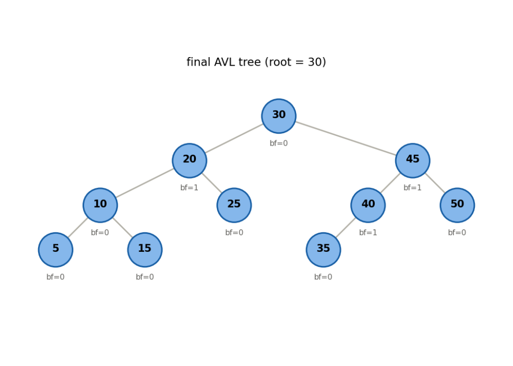
Avl Tree Visualization An AVL Tree is a special type of Binary Search Tree that automatically keeps itself balanced. A normal Binary Search Tree can provide very fast searching, insertion, and deletion when the tree remains balanced. In that situation, these operations can take O(log n) time. However, a normal Binary Search Tree does not automatically control its shape. If we insert values in a certain order, the tree can become very tall. When that happens, the tree can start behaving like a linked list, and searching can take O(n) time. An AVL Tree solves this problem by checking its balance after every insertion and deletion. When the tree becomes unbalanced, it changes its structure using rotations. In this article, we will learn how AVL Trees work, why we need them, how to calculate their balance factor, how rotations work, and how to implement an AVL Tree in C++. What Is a Binary Search Tree? Before understanding an AVL Tree, we need to understand a Binary Search Tree. A Binary Search Tree, usually called a BST, stores values according to a simple rule. Every value in the left subtree must be smaller than the current node. Every value in the right subtree must be larger than the current node. For example: 50 / \ 30 70 / \ / \ 20 40 60 80 The root contains 50. Values smaller than 50 go to the left. Values larger than 50 go to the right. The same rule continues inside every subtree. For example, 30 has 20 on its left because 20 is smaller than 30. It has 40 on its right because 40 is larger than 30. This structure allows us to search efficiently. Suppose we want to find 60. We start at 50. Since 60 is greater than 50, we move to the right. We reach 70. Since 60 is smaller than 70, we move to the left. We reach 60. We found the value after checking only a few nodes. The Problem With a Normal Binary Search Tree A Binary Search Tree does not automatically balance itself. Suppose we insert these values in this order: 10 20 30 40 50 The tree can become: 10 \ 20 \ 30 \ 40 \ 50 This tree still follows all the rules of a Binary Search Tree. However, the structure is inefficient. The tree has almost become a linked list. If we search for 50, we have to visit: 10 → 20 → 30 → 40 → 50 If the tree contains one million nodes and has this shape, a search could require almost one million comparisons. The search time becomes O(n). A balanced tree gives us a much smaller height. For one million nodes, a balanced tree can have a height close to log₂(1,000,000), which is about 20. This means we can search through a very large collection while checking only a small number of levels. What Is an AVL Tree? An AVL Tree keeps the Binary Search Tree rules while also keeping the tree balanced. AVL stands for Adelson Velsky and Landis, the names of the researchers who introduced this data structure. The main rule is simple. For every node, the height difference between the left subtree and the right subtree must not be greater than 1. The tree checks this difference using something called the balance factor. If the tree becomes unbalanced, the AVL Tree performs a rotation to fix its structure. The AVL Tree therefore combines two important ideas: Binary Search Tree + Automatic balancing = AVL Tree What Is Height? Height tells us how many levels exist below a node. For our implementation, we use the following definition: Empty tree = 0 New node = 1 For example: 50 / \ 30 70 The nodes 30 and 70 have height 1. The node 50 has height 2. Now consider: 50 / 30 / 20 The node 20 has height 1. The node 30 has height 2. The node 50 has height 3. We calculate the height of a node using: height = 1 + maximum(left height, right height) The 1 represents the current node. What Is the Balance Factor? The balance factor tells us whether a node has a balanced structure. We calculate it using: Balance Factor = Height of Left Subtree − Height of Right Subtree Suppose a node has: Left height = 3 Right height = 2 Then: Balance Factor = 3 − 2 = 1 The node is balanced. Now suppose we have: Left height = 3 Right height = 1 Then: Balance Factor = 3 − 1 = 2 The node is now unbalanced. An AVL Tree allows these balance factors: −1 0 +1 When the balance factor becomes: −2 or: +2 the node needs rebalancing. Why Does an AVL Tree Need Rotations? When we insert a new value, we can make one side of the tree taller than the other side. For example: 30 / 20 / 10 The left side has become much taller than the right side. The balance factor of 30 is: 2 The tree needs to change its structure. We call this structural change a rotation. A rotation moves nodes around while keeping the Binary Search Tree ordering correct. AVL Trees use four main cases: Left Left Right Right Left Right Right Left Left Left Case Consider inserting: 30 20 10 The tree becomes: 30 / 20 / 10 The new value moved left from 30 and then left again from 20. This creates the Left Left case. The balance factor of 30 becomes +2. We fix the tree using a right rotation. Before the rotation: 30 / 20 / 10 After the rotation: 20 / \ 10 30 The tree becomes balanced. Right Right Case Now consider inserting: 10 20 30 The tree becomes: 10 \ 20 \ 30 The new value moved right from 10 and then right again from 20. This creates the Right Right case. The balance factor of