
Type I and Type II Errors: Differences, Examples, and How to Reduce Them
Learn what Type I and Type II errors mean in statistics. Compare false positives and false negatives, understand alpha, beta and statistical power, and explore real-world and machine learning examples.
 Nov 15, 2026Published
11 min readReading time
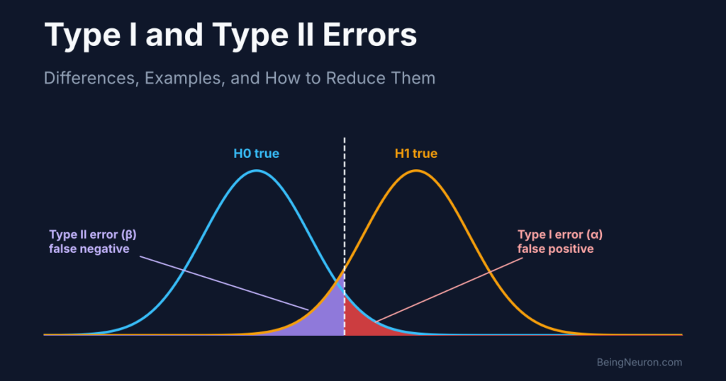
Imagine a medical test that tells a healthy person they have a disease. Now imagine the same test tells a person who has the disease that they are healthy. Both are incorrect decisions, but they are different kinds of mistakes.
In statistics, these mistakes are known as Type I and Type II errors. They occur when researchers use sample data to make a decision about a population through hypothesis testing. Understanding them helps researchers interpret evidence, design better experiments, and avoid misleading conclusions.
These ideas also connect to machine learning. False positives and false negatives appear in classification systems such as spam filters, fraud detection, and medical screening. The connection is useful, but the terms are not interchangeable in every context. This guide explains both the statistical definitions and their machine-learning counterparts.
What Are Type I and Type II Errors?
Type I and Type II errors are two possible mistakes in statistical hypothesis testing. To understand them, start with the two hypotheses used in a test.
The null hypothesis (H₀) is the starting claim. It often states that there is no effect, no difference, or no relationship. The alternative hypothesis (H₁) states that an effect, difference, or relationship exists.
For example, a research team tests whether a new medicine lowers blood pressure:
- Null hypothesis (H₀): The medicine does not lower blood pressure compared with the control treatment.
- Alternative hypothesis (H₁): The medicine lowers blood pressure compared with the control treatment.
After collecting sample data, the researchers decide whether to reject the null hypothesis or fail to reject it. Either decision can be right or wrong:
| Reality | Decision | Outcome |
|---|---|---|
| H₀ is true | Reject H₀ | Type I error |
| H₀ is true | Fail to reject H₀ | Correct decision |
| H₀ is false | Reject H₀ | Correct decision |
| H₀ is false | Fail to reject H₀ | Type II error |
Notice the wording: researchers usually say fail to reject the null hypothesis, not accept it. A test that does not find enough evidence against H₀ has not proved that H₀ is true.
Type I Error: A False Positive
A Type I error happens when a researcher rejects a null hypothesis that is actually true. The test reports evidence of an effect even though the effect is not present under the null hypothesis. This is commonly called a false positive.
Return to the medicine example. Suppose the medicine has no real effect, but the study produces a statistically significant result and the researchers reject H₀. They conclude that the medicine lowers blood pressure when it does not. That incorrect rejection is a Type I error.
What does alpha (α) mean?
The probability of a Type I error, when the null hypothesis is true and the test assumptions hold, is represented by alpha (α). Researchers choose a significance level before analyzing the results.
| Significance level | Nominal Type I error rate |
|---|---|
| α = 0.10 | 10% |
| α = 0.05 | 5% |
| α = 0.01 | 1% |
| α = 0.001 | 0.1% |
For example, setting α = 0.05 means that the testing procedure is designed to reject a true null hypothesis in 5% of repeated tests under the stated conditions. It does not mean there is a 5% probability that a particular research conclusion is wrong.
Type II Error: A False Negative
A Type II error happens when a researcher fails to reject a null hypothesis that is actually false. A real effect exists, but the test does not detect enough evidence for it. This is commonly called a false negative.
Suppose the medicine really does lower blood pressure, but the study has too few participants or measurements that vary widely. The test may not reach statistical significance. Researchers fail to detect the medicine’s real effect, producing a Type II error.
What does beta (β) mean?
The probability of a Type II error is represented by beta (β). Unlike a chosen significance level, beta depends on the specific alternative being considered and on the study design.
For example, β = 0.20 means that the test has a 20% probability of failing to reject H₀ for the particular effect size and assumptions used in the power calculation.
Type I vs Type II Errors: Key Differences
| Feature | Type I error | Type II error |
|---|---|---|
| Common name | False positive | False negative |
| What goes wrong? | Reject a true H₀ | Fail to reject a false H₀ |
| Symbol | α (alpha) | β (beta) |
| Simple interpretation | Report an effect that is not there | Miss an effect that is there |
| Possible consequence | False discovery or unnecessary action | Missed discovery or delayed action |
How to remember the difference
Think of a security alarm. A Type I-like mistake is an alarm that sounds when there is no intruder: a false alarm. A Type II-like mistake is an intruder entering without the alarm sounding: a missed detection.
- Type I: false alarm.
- Type II: missed alarm.
Alpha, Beta, and Statistical Power
Alpha and beta describe two different error probabilities. A related concept, statistical power, describes how likely a test is to detect a specified effect when that effect exists.
Statistical power = 1 − β
If β = 0.20, then power = 1 − 0.20 = 0.80, or 80%. Under the assumptions used to plan the test, this means an 80% chance of rejecting H₀ when the specified alternative is true.
| Term | Meaning |
|---|---|
| Alpha (α) | Probability of a Type I error under H₀ |
| Beta (β) | Probability of a Type II error for a specified alternative |
| Power (1 − β) | Probability of detecting that specified effect |
Power is not one universal property of a test. It changes with the effect size, sample size, data variability, significance level, and test design. Researchers often plan for 80% or 90% power, but the right target depends on the consequences of missing an effect.
Are Type I and Type II Errors Inversely Related?
There is often a trade-off between the two errors when the sample size and other design choices stay fixed. Lowering alpha makes it harder to reject H₀. This reduces the Type I error rate, but it can increase the chance of a Type II error.
For example, changing the significance level from 0.05 to 0.01 requires stronger evidence before rejecting the null hypothesis. That makes false alarms less likely, but a real effect may be harder to detect.
The trade-off is not unavoidable. Increasing the sample size can often improve power while keeping alpha at the chosen level. Better measurements, lower variability, and a more suitable study design can also help reduce both risks.
Real-World Examples of Type I and Type II Errors
1. Medical screening
A screening test may flag a healthy person as having a disease (false positive), or it may fail to flag a person who has the disease (false negative). The consequences differ: false positives can lead to anxiety and follow-up tests, while false negatives can delay diagnosis. These are diagnostic classification outcomes; they match Type I and Type II errors when expressed through a corresponding null-hypothesis decision.
2. Spam detection
A spam filter makes a false positive when it sends a legitimate email to the spam folder. It makes a false negative when a spam message reaches the inbox. The best balance depends on how users value catching spam versus avoiding misplaced messages.
3. Fraud detection
A bank’s system makes a false positive when it flags a legitimate transaction as fraud. It makes a false negative when it misses a fraudulent transaction. Both can be costly: one inconveniences customers, while the other may allow financial loss.
4. Courtroom decisions
As a simplified analogy, suppose the null hypothesis represents the claim that a defendant is innocent. Rejecting that hypothesis when the defendant is innocent resembles a Type I error. Failing to reject it when the defendant is guilty resembles a Type II error. Real legal systems involve standards and safeguards beyond statistical hypothesis testing, so this is an illustration rather than a literal statistical model of a trial.
5. Scientific research
A Type I error can lead researchers to report an effect that is not real. A Type II error can cause them to miss an effect that does exist. Both can misdirect later research, which is why study design, sample size, and transparent reporting matter.
How to Reduce Type I and Type II Errors
1. Choose an appropriate significance level
Choose alpha before analyzing the data and justify it based on the research question and the cost of a false positive. A smaller alpha controls Type I errors more strictly, but researchers should consider its effect on power.
2. Plan an adequate sample size
Small samples often make real effects harder to detect. A power analysis can estimate the sample size needed to detect an effect of practical importance at a chosen alpha and target power. A larger sample is useful only when the sampling and study design are also sound.
3. Improve the experimental design
Use suitable sampling, control important variables, define outcomes in advance, and choose a statistical test that matches the data and research question. Poor design can create bias that a larger sample will not fix.
4. Improve measurement quality
Unreliable instruments and inconsistent data collection increase noise. Clear procedures, calibrated equipment, and careful data checks can reduce unnecessary variability.
5. Account for multiple testing
Testing many hypotheses increases the chance of obtaining at least one false positive. Researchers may need procedures such as a family-wise error correction or false discovery rate control, depending on the study.
Type I and Type II Errors in Machine Learning
In binary classification, models can make false positive and false negative predictions. These outcomes are related to the ideas behind Type I and Type II errors, but the statistical definitions depend on how the hypotheses and positive class are defined.
For example, a fraud detection model predicts whether a transaction is fraudulent:
- False positive: the model predicts fraud for a legitimate transaction.
- False negative: the model predicts legitimate for a fraudulent transaction.
Understanding the confusion matrix
A confusion matrix compares predicted labels with actual labels. It contains four outcomes:
| Actual / Predicted | Predicted positive | Predicted negative |
|---|---|---|
| Actually positive | True positive (TP) | False negative (FN) |
| Actually negative | False positive (FP) | True negative (TN) |
These counts help calculate classification metrics. To understand how to evaluate a classifier in more detail, read our guide on evaluating a supervised learning model.
Connection to precision and recall
Precision asks how many predicted positives were actually positive:
Precision = TP / (TP + FP)
Recall asks how many actual positives the model successfully identified:
Recall = TP / (TP + FN)
High precision means fewer false alarms among positive predictions. High recall means fewer missed positive cases. In fraud detection, a team may prioritize recall to catch more fraud, while also monitoring false alarms that disrupt legitimate customers. You can also explore anomaly detection in machine learning, where unusual transactions may be flagged for investigation.
Model evaluation should use data that was not used to train the model. When comparing models, K-fold cross-validation can provide a more stable estimate of performance.
Python Example: Performing a Hypothesis Test
You can use Python’s SciPy library to run a two-sample hypothesis test. In this example, two independent groups represent measurements taken under a control condition and a treatment condition. The test evaluates whether their population means differ.
import numpy as np
from scipy.stats import ttest_ind

control = np.array([128, 132, 130, 127, 135, 129, 131, 126])
treatment = np.array([122, 125, 121, 124, 127, 123, 120, 126])

statistic, p_value = ttest_ind(
    treatment,
    control,
    equal_var=False
)

alpha = 0.05

print("Test statistic:", round(statistic, 3))
print("P-value:", round(p_value, 4))

if p_value < alpha:
    print("Reject the null hypothesis")
else:
    print("Fail to reject the null hypothesis")
The null hypothesis in this example says that the two population means are equal. The alternative says that they differ. The code uses Welch’s two-sample t-test, which does not assume equal population variances.
If the p-value is below 0.05, the test rejects the null hypothesis at the 5% significance level. If the null hypothesis is actually true, that decision would be a Type I error. If the p-value is 0.05 or higher, the test fails to reject the null hypothesis. If a real difference actually exists, that decision would be a Type II error.
Important: The result of one test does not tell you whether a Type I or Type II error actually occurred, because the true population condition is usually unknown. The significance level controls a long-run error rate under the null hypothesis; power analysis estimates the chance of detecting a specified real effect.
Frequently Asked Questions
What are Type I and Type II errors in statistics?
Type I error means rejecting a true null hypothesis. Type II error means failing to reject a false null hypothesis. They describe two different ways a hypothesis-testing decision can be wrong.
What is the difference between Type 1 and Type 2 errors?
Type 1 error is a false positive in the hypothesis-testing framework: a true null hypothesis is rejected. Type 2 error is a false negative: a false null hypothesis is not rejected.
How do you remember Type I and Type II errors?
Remember Type I as a false alarm and Type II as a missed alarm. A security alarm that sounds with no intruder illustrates the first; an alarm that misses an intruder illustrates the second.
Which error is worse?
Neither is always worse. The consequences depend on the application. Missing a serious disease may be more harmful than ordering an unnecessary follow-up test, while a high false-alarm rate may be especially disruptive in another setting.
Can Type I and Type II errors both be reduced?
Often, yes. Increasing sample size, improving measurement quality, and strengthening the study design can improve power while keeping the chosen significance level. No method guarantees that both error probabilities will be zero.
What is the relationship between alpha and beta?
Alpha is the Type I error probability under the null hypothesis. Beta is the Type II error probability for a specified alternative. Statistical power equals 1 − beta.
To understand how these errors affect different prediction methods, see our complete guide to machine learning models.
Conclusion
Type I and Type II errors describe two different mistakes in hypothesis testing. A Type I error rejects a true null hypothesis, while a Type II error fails to reject a false one. Alpha controls the Type I error rate, beta describes the Type II error probability for a specified alternative, and power measures the chance of detecting that effect.
These ideas also help explain false positives and false negatives in machine learning classification. Understanding which mistake matters most helps researchers design better experiments and helps developers evaluate models more responsibly.
This article is for educational purposes. Statistical conclusions depend on the study design, assumptions, and context in which a test is used.