
Deep Q-Networks (DQN) Explained: From Q-Learning to Deep Reinforcement Learning
Learn how a deep Q-network replaces the Q-table with a neural network, with experience replay, target networks and a tested PyTorch CartPole agent.
 Nov 20, 2026Published
22 min readReading time
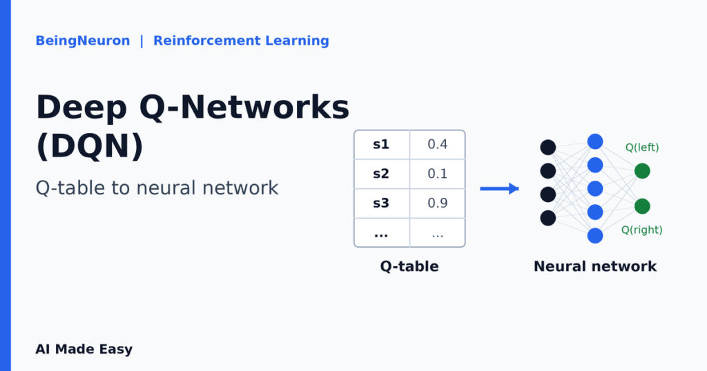
Q-learning stores one number for every state-action pair, and that works beautifully while the world is small. Now give the agent a different job: balance a pole on a moving cart. The cart’s position, its speed, the pole’s angle and the pole’s rotation speed are all continuous numbers, so the agent can visit an endless supply of slightly different states and almost never see the same one twice. A table with one row per state cannot even be written down, let alone filled in.
The deep Q-network (DQN) solves this by replacing the table with a neural network. Instead of looking up a stored value, the agent asks the network to compute it, and because networks generalize, a state the agent has never visited still gets a sensible answer. But a neural network trained on Q-learning targets is notoriously unstable, so DQN adds two stabilizers: experience replay and a target network. This guide explains why the table fails, how the network takes its place, what the loss function is, why each stabilizer is needed, and then builds a complete DQN in PyTorch that learns CartPole with Gymnasium. It ends with the limitations, including results from my own runs that show how fragile deep RL can be.
This is the third algorithm in our value-based sequence. It assumes you know the update rule from Q Learning Update Rule Explained: Formula, Algorithm & Python Example and the on-policy idea from SARSA Algorithm Explained: On-Policy Reinforcement Learning. For the foundations, see What Is Reinforcement Learning? A Complete Guide.
Why Q-Learning Uses a Q-Table, and Where It Breaks
Tabular Q-learning keeps one value Q(s, a) per state and action, stored in a table with a row for each state and a column for each action. The update rule edits a single cell after each step. The table has two properties that make the algorithm simple and reliable: every state-action pair is learned independently, and lookups are exact.
Those same properties become the problem as environments grow.
- The table gets too big. Its size is the number of states times the number of actions. A video game screen of 84 × 84 pixels, with 256 brightness levels per pixel and four stacked frames (the input used in the original DQN work), has roughly 1068,000 possible states. No memory could hold that table.
- Continuous states cannot be enumerated. CartPole’s four state variables are real numbers, so there are infinitely many states. You can force a table by cutting each variable into bins, but fine bins make the table huge and coarse bins throw away information.
- Nothing is shared between states. If the pole is leaning at 3.00° and the agent learned to push left, a table knows nothing about 3.01°. Every state must be visited and learned on its own, which is hopelessly slow when states are almost identical.
What we want is a function that takes a state and returns action values, and that treats similar states similarly. That is exactly what a neural network provides.
From Q-Learning to Deep Q-Networks
A DQN keeps Q-learning’s core idea, learning action values from a target built out of reward plus the discounted best next value, but stores the values in the weights of a neural network. We write the network’s estimate as Q(s, a; θ), where θ stands for all the network’s weights. Instead of overwriting a table cell, training nudges θ so that the network’s output moves toward the target. Since every state passes through the same weights, learning from one state improves the estimate for similar ones.
The relationship in one sentence: DQN is Q-learning with function approximation, where gradient descent on a neural network replaces the direct edit of a table cell. The target r + γ · max Q(s′, a′) is the same. What changes is how the estimate is stored and updated, and that change creates the stability problems the rest of this article addresses.
| Aspect | Tabular Q-learning | Deep Q-Network |
|---|---|---|
| Where values live | A table: one cell per state-action pair | Weights θ of a neural network |
| How an update works | Edit one cell directly | Gradient step that changes all the weights a little |
| State space | Small and discrete | Large or continuous, including images |
| Generalization | None: each state learned separately | Similar states share what the network learned |
| Training data | Each experience used once, in order | Experiences stored and replayed in random batches |
| Target | Computed from the same table | Computed from a separate, slowly updated target network |
| Convergence | Guaranteed under standard conditions | No general guarantee; can be unstable |
The Architecture of a Deep Q-Network
The key design choice is on the output side. The network takes the state as input and produces one Q-value for every action in a single forward pass. With two actions, the output has two numbers. The agent then reads off the best action with an argmax. This is far more efficient than feeding in a state and an action and getting back one number, because a single pass gives every action value at once.
For CartPole, the input is four numbers: cart position, cart velocity, pole angle and pole angular velocity. The output is two Q-values: one for pushing the cart left and one for pushing it right. Two hidden layers sit between them.
The hidden layers use the ReLU activation, which is standard for networks like this. If you want a refresher on how such layers work, see Multilayer Perceptron. When the input is an image rather than a short list of numbers, the same design is used with convolutional layers, as in the original paper, which stacked four preprocessed 84 × 84 frames as input.
How the Network Learns: The DQN Loss Function
Supervised networks learn from labeled examples. A DQN has no labels, so it manufactures its own: for each stored experience, it builds a target from the reward and the network’s own estimate of the next state, exactly like the TD target in Q-learning. Training then makes the prediction match that target.
For one experience (s, a, r, s′), the target is:
| Symbol | Meaning |
|---|---|
| θ | The weights of the online network, the one being trained and used to act. |
| θ− | The weights of the target network, a frozen copy of θ that changes only occasionally. |
| Q(s, a; θ) | The online network’s current prediction for action a in state s. |
| r, γ | The reward received and the discount factor, as in Q-learning. |
| maxa′ Q(s′, a′; θ−) | The best next-state value according to the target network. |
| y | The target: the number the prediction should move toward. It is treated as a constant, so no gradient flows through it. |
| E[ … ] | The average over a minibatch of stored experiences. |
A worked example. Take γ = 0.99 and a stored experience with reward r = 1. The target network says the next state’s action values are 10.2 and 9.7, so the best one is 10.2. The target is y = 1 + 0.99 × 10.2 = 11.098. Suppose the online network currently predicts Q(s, a) = 10.5. The error is 11.098 − 10.5 = 0.598, and the squared error is about 0.3576. Gradient descent changes θ to shrink that number. If instead s′ were terminal, the target would be just y = 1, the error would be 1 − 10.5 = −9.5, and the squared error would be 90.25. That large gap would drive a strong correction.
Two practical notes. First, the code below uses the Huber loss (smooth_l1_loss) instead of a pure squared error. It behaves like squared error for small errors but grows only linearly for large ones, so a few extreme targets cannot cause huge gradient steps. The original paper reached a similar goal by clipping the error term. Second, only the online network’s prediction Q(s, a; θ) is trained. The target y is computed under torch.no_grad() and held fixed.
Experience Replay
If the agent trained on each experience immediately, in the order it happened, two problems would appear. Consecutive steps are strongly correlated: ten frames of the pole slowly tilting look almost identical, but neural network training assumes samples are roughly independent. And each experience would be used once and thrown away, even though it may be rare and valuable.
Experience replay fixes both. The agent stores every transition (s, a, r, s′, done) in a fixed-size memory called the replay buffer. When it is time to learn, it draws a random minibatch from the buffer and trains on that. The original DQN paper drew samples uniformly at random, and so does the code below.
Why random sampling helps training
- It breaks correlation. A random batch mixes experiences from many different moments and situations, which looks much more like the independent data that gradient descent expects.
- It reuses data. Each experience can contribute to many updates, which matters because interacting with an environment is often the expensive part.
- It smooths out drift. Without replay, the agent’s current behavior determines its training data, so a change in behavior changes the data, which changes the network, which changes the behavior. A mixed buffer dampens that feedback loop.
- It prevents forgetting. Old situations stay in the mix instead of being overwritten by whatever the agent is doing right now.
Replay works because DQN is off-policy, as you saw in the on-policy versus off-policy comparison in the SARSA article. A transition collected by an older, more random version of the policy is still a valid sample for the Q-learning target, since that target uses the max rather than the action actually taken next.
The Target Network
In supervised learning the labels sit still while the network learns. In DQN the target y is computed by the same network that is being trained. Every update changes θ, which changes the targets, which the network is chasing in the next update. It is like trying to hit a target that moves every time you move your aim, and this feedback can make training oscillate or diverge.
The fix is a second network, the target network, with its own weights θ−. It starts as an exact copy of the online network and is used only to compute the max term in the target. Its weights are frozen while the online network trains, and every C steps they are overwritten with a fresh copy of θ. Between copies the target is stable, so the online network gets a steady goal for a while. In the code below, C is 250 steps. (Some implementations instead blend the weights a little every step, called a soft update.)
Epsilon-Greedy Exploration in DQN
DQN explores with the same epsilon-greedy rule you met in Q-learning and SARSA. With probability ε the agent picks a random action. Otherwise it feeds the state through the network and takes the action with the largest Q-value. Early on, the network’s outputs are meaningless, so a high ε keeps the agent from acting on noise and fills the replay buffer with varied experience. The code decays ε linearly from 1.0 to 0.05 over the first 10,000 steps and then holds it at 0.05. For the mechanics and probabilities of epsilon-greedy, see the epsilon-greedy section of the SARSA article.
The Complete DQN Training Process
- Initialize. Create the online network with random weights, copy it into the target network, and create an empty replay buffer.
- Observe the state from the environment.
- Choose an action with epsilon-greedy using the online network.
- Act and observe the reward, the next state, and whether the episode ended.
- Store the transition (s, a, r, s′, done) in the replay buffer.
- Sample a random minibatch from the buffer (once it holds enough experience).
- Compute targets y = r + γ · max Q(s′, a′; θ−) with the target network, or y = r for terminal transitions.
- Take a gradient step on the loss between Q(s, a; θ) and y to update the online network.
- Sync the target network every C steps by copying θ into θ−.
- Repeat from step 2, decaying ε as training proceeds.
DQN pseudocode
initialize online network Q(s, a; theta) with random weights
initialize target network with theta_minus = theta
initialize empty replay buffer D

for each step:
    choose a: random with probability epsilon, else argmax over a' of Q(s, a'; theta)
    take a, observe r, s_next, done
    store (s, a, r, s_next, done) in D
    s = s_next  (reset the environment if the episode ended)

    if D holds enough transitions:
        sample a random minibatch (s, a, r, s_next, done) from D
        y = r + gamma * max over a' of Q(s_next, a'; theta_minus) * (1 - done)
        loss = (y - Q(s, a; theta))^2           # averaged over the minibatch
        update theta by gradient descent on loss

    every C steps:
        theta_minus = theta
Implementing a Deep Q-Network in PyTorch
We train a DQN on CartPole-v1, a standard Gymnasium environment. A pole is hinged to a cart, and the agent pushes the cart left or right to keep the pole upright. The agent receives +1 reward for every step the pole stays up. An episode ends if the pole tilts too far or the cart leaves the track, and it is cut off at 500 steps, so the maximum return is 500.
Installation. Run pip install torch gymnasium numpy. Copy the stages below, in order, into one file named dqn_cartpole.py. I ran this exact script on a single CPU core (no GPU needed) with Python 3.12.3, PyTorch 2.15.0, Gymnasium 1.4.0 and NumPy 2.5.4. Training takes a few minutes.
Stage 1: Imports and hyperparameters
import random
from collections import deque

import gymnasium as gym
import numpy as np
import torch
import torch.nn as nn
import torch.nn.functional as F

SEED = 0
ENV_NAME = "CartPole-v1"

GAMMA = 0.99               # discount factor
LEARNING_RATE = 5e-4
BATCH_SIZE = 64
BUFFER_SIZE = 50_000
LEARNING_STARTS = 1_000    # collect this many steps before any training
TARGET_UPDATE_EVERY = 250  # copy online weights into the target network
EPSILON_START, EPSILON_END = 1.0, 0.05
EPSILON_DECAY_STEPS = 10_000
TOTAL_STEPS = 60_000
These constants control the whole experiment. GAMMA is γ. BUFFER_SIZE caps the replay memory, and when it is full the oldest transitions are dropped. LEARNING_STARTS delays training until the buffer holds some varied experience. TARGET_UPDATE_EVERY is C. The ε values define the exploration schedule.
Stage 2: The Q-network
class QNetwork(nn.Module):
    """State in, one Q-value per action out."""

    def __init__(self, state_dim, n_actions, hidden=128):
        super().__init__()
        self.net = nn.Sequential(
            nn.Linear(state_dim, hidden), nn.ReLU(),
            nn.Linear(hidden, hidden), nn.ReLU(),
            nn.Linear(hidden, n_actions),
        )

    def forward(self, x):
        return self.net(x)
This is the network from Figure 2. It takes state_dim numbers (4 for CartPole), passes them through two hidden layers of 128 units with ReLU, and outputs n_actions numbers (2). The final layer has no activation, because Q-values are unbounded real numbers.
Stage 3: The replay buffer
class ReplayBuffer:
    def __init__(self, capacity):
        self.memory = deque(maxlen=capacity)

    def push(self, state, action, reward, next_state, terminated):
        self.memory.append((state, action, reward, next_state, terminated))

    def sample(self, batch_size):
        batch = random.sample(self.memory, batch_size)      # uniform random sample
        states, actions, rewards, next_states, dones = zip(*batch)
        return (
            torch.as_tensor(np.array(states), dtype=torch.float32),
            torch.as_tensor(actions, dtype=torch.int64).unsqueeze(1),
            torch.as_tensor(rewards, dtype=torch.float32).unsqueeze(1),
            torch.as_tensor(np.array(next_states), dtype=torch.float32),
            torch.as_tensor(dones, dtype=torch.float32).unsqueeze(1),
        )

    def __len__(self):
        return len(self.memory)
A deque with maxlen automatically discards the oldest transition when full. push stores one experience. sample draws a random batch with random.sample, then regroups the tuples into one tensor per field. The unsqueeze(1) calls reshape actions, rewards and done flags to a column of shape (batch, 1), so they line up with the network output later.
Stage 4: Exploration
def epsilon_at(step):
    fraction = min(1.0, step / EPSILON_DECAY_STEPS)
    return EPSILON_START + fraction * (EPSILON_END - EPSILON_START)


def select_action(online_net, state, epsilon, n_actions):
    if random.random() < epsilon:
        return random.randrange(n_actions)                   # explore
    with torch.no_grad():
        q_values = online_net(torch.as_tensor(state, dtype=torch.float32).unsqueeze(0))
    return int(q_values.argmax(dim=1).item())                # exploit
epsilon_at slides ε linearly from 1.0 to 0.05 over the first 10,000 steps. select_action either picks a random action or runs the state through the network and takes the argmax. The unsqueeze(0) adds a batch dimension of 1, and torch.no_grad() skips gradient tracking because this is only inference.
Stage 5: One learning step
def optimize(online_net, target_net, optimizer, buffer):
    states, actions, rewards, next_states, dones = buffer.sample(BATCH_SIZE)

    # Q(s, a) from the online network, for the actions that were actually taken
    q_sa = online_net(states).gather(1, actions)

    # Target y = r + gamma * max_a' Q_target(s', a'); no future reward if terminated
    with torch.no_grad():
        next_max = target_net(next_states).max(dim=1, keepdim=True).values
        targets = rewards + GAMMA * next_max * (1.0 - dones)

    loss = F.smooth_l1_loss(q_sa, targets)                   # Huber loss
    optimizer.zero_grad()
    loss.backward()
    nn.utils.clip_grad_norm_(online_net.parameters(), 10.0)
    optimizer.step()
    return loss.item()
This function is the heart of DQN. It samples a minibatch. The network outputs a Q-value for every action, and gather(1, actions) picks out the one for the action actually taken, which gives Q(s, a; θ). Inside torch.no_grad(), the target network computes the best next value, and the target is r + γ · max Q, multiplied by (1 - dones) so that terminal transitions get no future term. Then the Huber loss compares prediction with target, backward() computes gradients, gradient clipping caps their size for safety, and the optimizer takes one step.
Stage 6: The training loop
def train(seed=SEED, total_steps=TOTAL_STEPS, log=True):
    random.seed(seed)
    np.random.seed(seed)
    torch.manual_seed(seed)

    env = gym.make(ENV_NAME)
    state_dim = env.observation_space.shape[0]
    n_actions = env.action_space.n

    online_net = QNetwork(state_dim, n_actions)
    target_net = QNetwork(state_dim, n_actions)
    target_net.load_state_dict(online_net.state_dict())
    optimizer = torch.optim.Adam(online_net.parameters(), lr=LEARNING_RATE)
    buffer = ReplayBuffer(BUFFER_SIZE)

    state, _ = env.reset(seed=seed)
    episode_return, episode_returns = 0.0, []

    for step in range(1, total_steps + 1):
        epsilon = epsilon_at(step)
        action = select_action(online_net, state, epsilon, n_actions)
        next_state, reward, terminated, truncated, _ = env.step(action)

        # Store 'terminated' (a real failure), not 'truncated' (the 500-step time limit)
        buffer.push(state, action, reward, next_state, float(terminated))
        state = next_state
        episode_return += reward

        if len(buffer) >= LEARNING_STARTS:
            optimize(online_net, target_net, optimizer, buffer)

        if step % TARGET_UPDATE_EVERY == 0:
            target_net.load_state_dict(online_net.state_dict())

        if terminated or truncated:
            episode_returns.append(episode_return)
            episode_return = 0.0
            state, _ = env.reset()
            if log and len(episode_returns) % 25 == 0:
                recent = np.mean(episode_returns[-25:])
                print(f"episode {len(episode_returns):4d} | step {step:6d} | "
                      f"epsilon {epsilon:.2f} | avg return (last 25) {recent:6.1f}")

    env.close()
    return online_net, episode_returns
Setup comes first: seeds for reproducibility, the environment, two networks (the target starts as a copy of the online one through load_state_dict), an Adam optimizer on the online network only, and the buffer. Each step then follows the process above: pick an action, step the environment, store the transition, train once the buffer has enough data, and every 250 steps copy the weights into the target network. When an episode ends, the code records its return and resets the environment.
One detail deserves attention. Gymnasium reports two kinds of episode end. terminated means a real failure, like the pole falling. truncated means the time limit of 500 steps was hit while the pole was still up. A truncated state still has future value, so the code stores only terminated as the done flag. Treating truncation as failure would wrongly teach the agent that surviving to step 500 is a dead end.
Stage 7: Evaluate the trained agent
def evaluate(online_net, episodes=20, seed=1234):
    env = gym.make(ENV_NAME)
    returns = []
    for i in range(episodes):
        state, _ = env.reset(seed=seed + i)
        done, total = False, 0.0
        while not done:
            with torch.no_grad():
                q = online_net(torch.as_tensor(state, dtype=torch.float32).unsqueeze(0))
            state, reward, terminated, truncated, _ = env.step(int(q.argmax(dim=1).item()))
            total += reward
            done = terminated or truncated
        returns.append(total)
    env.close()
    return returns


if __name__ == "__main__":
    model, _ = train()
    scores = evaluate(model)
    print(f"\nGreedy evaluation over {len(scores)} episodes: "
          f"mean = {np.mean(scores):.1f}, min = {np.min(scores):.0f}, max = {np.max(scores):.0f}")
Evaluation is deliberately different from training. It uses a fresh environment with different starting conditions (seeds 1234 to 1253), always takes the greedy action with no exploration, and does no learning. This measures what the agent actually learned instead of how well it performed while exploring. Running the script with seed 0 produced:
episode   25 | step    670 | epsilon 0.94 | avg return (last 25)   26.8
episode   50 | step   1270 | epsilon 0.88 | avg return (last 25)   24.0
episode   75 | step   1823 | epsilon 0.83 | avg return (last 25)   22.1
episode  100 | step   2900 | epsilon 0.72 | avg return (last 25)   43.1
episode  125 | step   3866 | epsilon 0.63 | avg return (last 25)   38.6
episode  150 | step   5813 | epsilon 0.45 | avg return (last 25)   77.9
episode  175 | step   8114 | epsilon 0.23 | avg return (last 25)   92.0
episode  200 | step  11444 | epsilon 0.05 | avg return (last 25)  133.2
episode  225 | step  15057 | epsilon 0.05 | avg return (last 25)  144.5
episode  250 | step  19728 | epsilon 0.05 | avg return (last 25)  186.8
episode  275 | step  25675 | epsilon 0.05 | avg return (last 25)  237.9
episode  300 | step  32263 | epsilon 0.05 | avg return (last 25)  263.5
episode  325 | step  42759 | epsilon 0.05 | avg return (last 25)  419.8
episode  350 | step  49384 | epsilon 0.05 | avg return (last 25)  265.0
episode  375 | step  59506 | epsilon 0.05 | avg return (last 25)  404.9

Greedy evaluation over 20 episodes: mean = 500.0, min = 500, max = 500Reading the Results Honestly
On seed 0 the greedy agent balanced the pole for the full 500 steps in all 20 evaluation episodes. But that is one run, and it deserves context, because deep RL results are much noisier than tabular ones.
- The training curve is bumpy. Look at the log: the 25-episode average reached 419.8, fell to 265.0, then recovered to 404.9. Even with replay and a target network, performance can swing during training.
- Seeds matter a lot. I ran seeds 0 to 4 with these exact settings and evaluated each greedily over 20 episodes. The mean scores were 500.0, 500.0, 286.2, 500.0 and 353.4. Three of five seeds balanced the pole perfectly, and two learned a decent but incomplete policy.
- Hyperparameters matter a lot. My first attempt used a learning rate of 1e-3, a target sync every 500 steps and 40,000 steps. It reached a greedy mean of only 145.3 on seed 0. I then tried three alternatives on seed 0 (60,000 steps each). The settings used here scored 500.0. A slower ε decay with sync every 500 steps scored 86.0, and a learning rate of 1e-3 with sync every 100 steps scored 194.4.
Two honest caveats. I chose these settings after seeing seed 0’s results, so seed 0 is not an unbiased test, and seeds 1 to 4 are the fairer check. And five seeds is a small sample, so treat these numbers as an illustration of variability, not a benchmark. If your run gives different numbers, that is normal. Your NumPy and PyTorch versions, and your hardware, will change random streams.
Q-Learning vs DQN
The two share an update target, but they differ in nearly everything around it. The table in the “From Q-Learning to Deep Q-Networks” section compares them side by side. The short version: use tabular Q-learning when the state space is small and discrete, because it is simple, fast and has convergence guarantees. Use a DQN when states are large or continuous and you can afford to tune for stability. Both are off-policy, and both learn action values, so they share a key limitation: they pick actions by taking a max over a discrete set of actions.
Limitations and Common Training Problems
| Problem | What it looks like | Typical remedies |
|---|---|---|
| Instability and divergence | Returns swing up and down, or Q-values blow up. It stems from combining a neural network, bootstrapped targets and off-policy data, sometimes called the “deadly triad”. | Target network, smaller learning rate, gradient clipping, Huber loss |
| Overestimation | The max over noisy estimates is biased upward, so values become too optimistic. | Double DQN, which selects the best next action with one network and evaluates it with the other |
| Sensitivity to hyperparameters | Small changes in learning rate or sync interval change results a lot, as the runs above show. | Careful tuning, multiple seeds, logging |
| Sample inefficiency | Many thousands of steps to learn even simple tasks. | Prioritized replay, larger replay buffers, better exploration |
| Poor exploration | Epsilon-greedy explores blindly, so sparse-reward tasks can stall. | Better exploration strategies, reward shaping |
| Discrete actions only | The max over actions requires a small, finite action set. Continuous controls such as torque cannot be handled directly. | Policy-based methods, which we cover next in this series |
| Wrong handling of episode ends | The agent seems to avoid reaching the time limit, because truncation was treated as failure. | Store terminated, not truncated, as the done flag |
Several well-known improvements address these issues, including Double DQN, prioritized experience replay and dueling networks. They are good topics for further reading once you are comfortable with the basic algorithm.
Where DQN Is Used
The best-documented success is the original work: a single DQN, receiving only screen pixels and the game score, reached a level comparable to a professional human games tester across a set of 49 Atari 2600 games, using the same algorithm, architecture and hyperparameters for every game (Mnih et al., Nature, 2015). Beyond that, DQN and its variants are widely used as baselines in research on game-playing agents and discrete-control tasks. For a broader and honest look at where reinforcement learning is applied, see Applications of Reinforcement Learning: 10 Real-World Examples.
Frequently Asked Questions
What is a deep Q-network?
A deep Q-network is a neural network that estimates the Q-value of every action for a given state. It is trained with a Q-learning target and uses experience replay and a target network to stay stable.
What is the difference between Q-learning and DQN?
Q-learning stores values in a table and edits one cell per update. DQN stores values in neural network weights, trains them by gradient descent on a loss, and adds replay and a target network because that training is less stable.
Why does DQN need a target network?
Without one, the network’s own changing predictions form the training targets, so the target moves every time the weights change. A target network is a slowly updated copy that keeps the target steady between syncs.
Why does DQN use experience replay?
Consecutive experiences are highly correlated and would otherwise be used only once. Replay stores them and trains on random minibatches, which reduces correlation and reuses data.
Is DQN on-policy or off-policy?
Off-policy. The target uses the maximum over next actions, so it learns about the greedy policy while the agent acts with an epsilon-greedy one, which also lets it learn from replayed older experience.
Can DQN handle continuous actions?
Not directly, because it takes a max over a finite set of actions. Policy-based methods are the usual choice for continuous control.
Conclusion and Next Steps
A DQN is Q-learning with the table swapped for a neural network, plus two ideas that make that swap workable: replay to decorrelate and reuse data, and a target network to stop the target chasing the prediction. You have seen the loss with real numbers, built the whole agent in PyTorch, trained it on CartPole, and seen that results vary across seeds and settings, which is typical of deep RL.
To practice, change one setting at a time in the script (target sync interval, learning rate, buffer size), run several seeds, and compare the greedy evaluation scores. To review the foundations, revisit Q Learning Update Rule Explained: Formula, Algorithm & Python Example and SARSA Algorithm Explained: On-Policy Reinforcement Learning.
DQN still relies on estimating action values and picking the best one. The next article in this series, Policy Gradient Methods Explained: Learning Policies Directly, drops that requirement and trains the policy itself, which is what makes continuous actions and stochastic behavior natural.