Unsupervised Learning Project: Customer Segmentation with Python

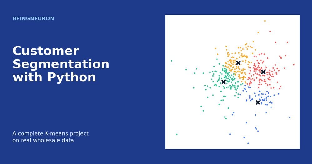
Customer segmentation with Python means grouping customers by how they behave so that a business can treat each group differently. It is the most common real-world use of clustering, and it makes a good capstone for this series because it uses almost everything you have learned: feature scaling, distance, K-means, choosing K, evaluation without labels, and PCA for visualization.

In this project you will work with a real public dataset of wholesale customers, clean and transform it, build K-means segments, check them with internal metrics, plot them, and turn them into business conclusions. You get one complete script that runs from top to bottom. If you are new to the method, read What Is Unsupervised Learning? and K-Means Clustering Explained first.

The Business Problem

A wholesale distributor sells to many different clients: restaurants, hotels, cafes, and retail shops. Each client buys a different mix of products. Treating all of them the same wastes effort. Sales visits, delivery schedules, discounts, and stock planning work better when they match what a group of customers actually needs.

The question for this project is: can we group these customers into a small number of segments based on their annual spending across product categories, and can each segment be described well enough to act on?

This is a clustering task because we have no predefined segment labels. We want the data to suggest the groups.

Dataset Selection and Source

The project uses the Wholesale Customers dataset from the UCI Machine Learning Repository, a public dataset donated by Margarida G. M. S. Cardoso (UCI Machine Learning Repository, dataset 292: archive.ics.uci.edu/dataset/292/wholesale+customers). It describes 440 clients of a wholesale distributor in Portugal.

I chose it for four reasons: it is real and freely available, it is small enough to run in seconds, it has no missing values, and its columns have a clear business meaning. It does not need a login to download.

Column	Meaning	Used for clustering?
Channel	Customer channel: 1 = Horeca (hotel, restaurant, cafe), 2 = Retail	No. Kept as an outside reference.
Region	Customer region code (1, 2, or 3)	No. A category, not spending.
Fresh	Annual spending on fresh products	Yes
Milk	Annual spending on milk products	Yes
Grocery	Annual spending on grocery products	Yes
Frozen	Annual spending on frozen products	Yes
Detergents_Paper	Annual spending on detergents and paper products	Yes
Delicassen	Annual spending on delicatessen products	Yes

The script reads the file directly from a public GitHub copy hosted in the PyCaret repository, and it uses a local file named wholesale-customers.csv if one is present. You can also download the original file from the UCI page and place it next to the script. The script checks that the data has the expected shape, 440 rows and 8 columns, as its first output line confirms.

Choosing the Features

The six spending columns are the behavior we want to segment on, so they are the clustering features. Channel and Region are categorical codes, and K-means averages numbers, so it would treat “Region 3” as three times “Region 1”, which has no meaning. They are excluded.

Channel deserves a closer look. It is excluded from clustering on purpose, so we can use it later as an independent check. If our segments, which never saw Channel, still line up with Channel in a sensible way, that is encouraging evidence that they capture real differences. It is not a ground truth, because Horeca and Retail are not the only possible segments, but it is a useful sanity check.

Exploratory Data Analysis

Before clustering, look at the data. The first output block shows that there are no missing values and no duplicate rows, so no cleaning is needed beyond transformation. Next, look at how each spending variable is distributed.

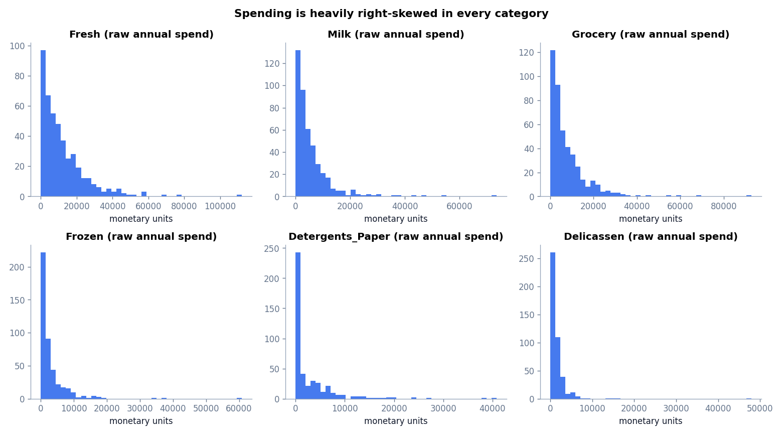
Every category is strongly right-skewed. The skewness values in the output range from 2.56 for Fresh to 11.15 for Delicassen, where a value near zero would indicate a symmetric distribution. Most customers spend modest amounts, and a few spend a great deal.

This matters for K-means. A handful of very large spenders would pull centroids toward them and could produce a cluster that contains only extreme customers. Standardizing alone does not fix skew.

Cleaning and Transforming the Data

There are two preprocessing steps.

1. Log transform. Apply log(1 + x) to each spending column. The log compresses large values, so a customer who spends 100,000 is no longer 100 times farther from the crowd than a customer who spends 1,000. Using log1p instead of log is safe if any value is zero. After the transform, skewness falls to between −1.58 and −0.22, which is much closer to symmetric. Fresh and Delicassen are still moderately skewed, now with a long tail of very small values.
2. Standardization. Rescale every transformed feature to mean 0 and standard deviation 1 with StandardScaler, so that no category dominates the distance calculation.

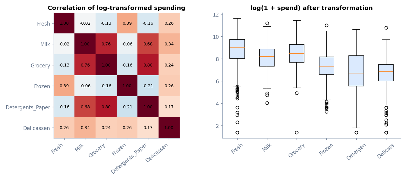
The correlation heatmap already tells a story. Customers who spend heavily on Milk also tend to spend heavily on Grocery and on Detergents and Paper. Those three categories form a related block, while Fresh and Frozen behave differently. K-means will use these relationships to separate customer types.

Notice what the pipeline does not do. It does not remove the high spenders. They are real customers, and the log transform handles their influence. Always document such decisions.

Choosing the Number of Clusters

The script fits K-means for K from 2 to 8 and records three numbers: inertia, silhouette score, and the Davies-Bouldin index. The silhouette score (higher is better) was explained in the K-means article. The Davies-Bouldin index compares within-cluster spread with between-cluster distance, and lower is better.

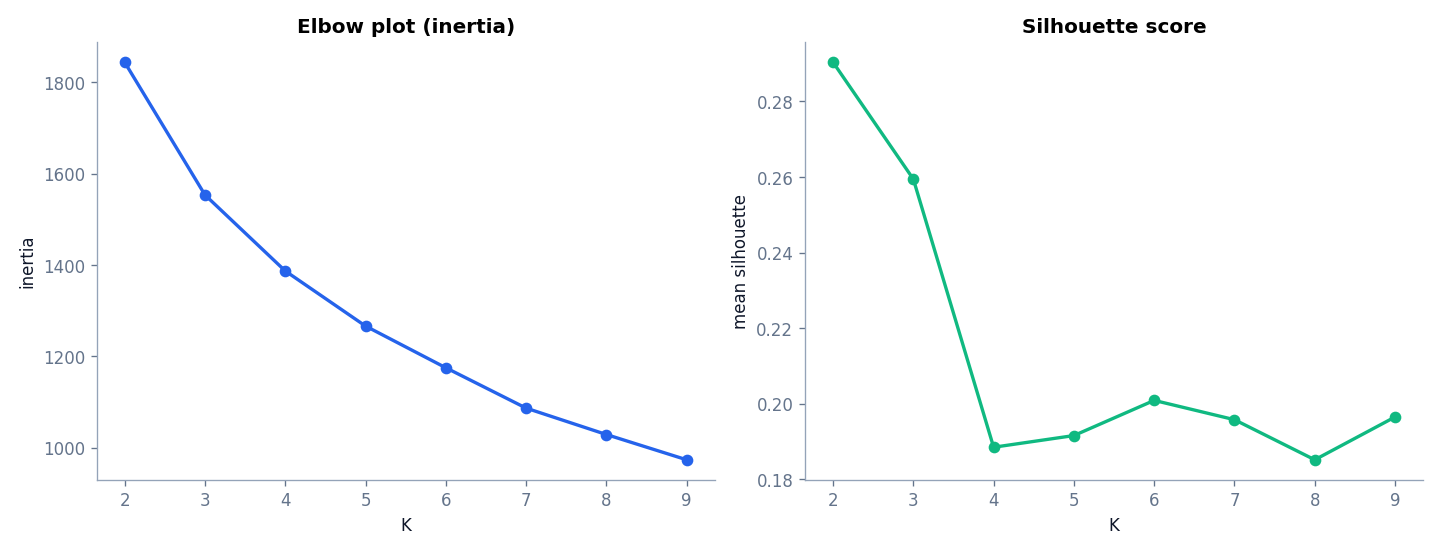
Here is what the numbers say:

• Inertia falls smoothly from 1,844 at K = 2 to 1,029 at K = 8. There is no sharp elbow.
• The silhouette score is highest at K = 2 (0.290) and is only about 0.19 to 0.20 for K from 4 to 8.
• Davies-Bouldin is lowest at K = 3 (1.341) and K = 2 (1.352).

These are weak scores. Silhouette values around 0.2 mean the clusters overlap considerably. Real customers do not fall into neat islands. They form a continuum, and the segments are a convenient way of cutting it. That is an honest finding, and it is worth saying clearly in any report.

Why this project uses K = 4

If we chose K purely by silhouette, we would choose K = 2. That split mostly separates two broad customer types, and it is probably too coarse to act on. A business that wants to tailor offers will often prefer a few more groups, as long as they are distinguishable and not tiny. This is a judgment call, not a mathematical result, and it carries a cost: K = 4 has a lower silhouette score (0.188) than K = 2 or 3. We accept that cost because four segments gave the clearest business descriptions in the next steps. If you prefer a more conservative model, change K = 4 in the script to 2 or 3 and compare.

The Complete Python Project

Copy the code below into a file named customer_segmentation.py. You need Python 3.9 or newer and the packages numpy, pandas, matplotlib, and scikit-learn.

How to run it:

1. Create a folder and, optionally, a virtual environment: python -m venv venv, then activate it.
2. Install the packages: pip install numpy pandas matplotlib scikit-learn.
3. Save the code as customer_segmentation.py. If you downloaded the CSV from the UCI repository, save it in the same folder as wholesale-customers.csv (the column names must match the table above). Otherwise the script downloads the public copy.
4. Run python customer_segmentation.py. The text output prints in the terminal and a window with the PCA plot opens.

"""Customer segmentation with K-means on the UCI Wholesale Customers dataset."""
import os
import numpy as np
import pandas as pd
import matplotlib.pyplot as plt
from sklearn.preprocessing import StandardScaler
from sklearn.cluster import KMeans
from sklearn.decomposition import PCA
from sklearn.metrics import silhouette_score, davies_bouldin_score

URL = "https://raw.githubusercontent.com/pycaret/pycaret/master/datasets/wholesale.csv"
LOCAL = "wholesale-customers.csv"   # or point this at a copy downloaded from the UCI repository

# 1. Load data (same 440 rows and 8 columns as the UCI file).
df = pd.read_csv(LOCAL if os.path.exists(LOCAL) else URL, encoding="utf-8-sig")
print("Shape:", df.shape)
print("Missing values:", int(df.isna().sum().sum()), " Duplicate rows:", int(df.duplicated().sum()))

# 2. Choose features. Channel and Region are categorical codes, so we keep them OUT of clustering
#    and use Channel later as an outside reference.
spend_cols = ["Fresh", "Milk", "Grocery", "Frozen", "Detergents_Paper", "Delicassen"]
print("\nSkewness before transform:")
print(df[spend_cols].skew().round(2).to_string())

# 3. Reduce skew with log(1 + x), then standardize.
X_log = np.log1p(df[spend_cols])
print("\nSkewness after log transform:")
print(X_log.skew().round(2).to_string())
X = StandardScaler().fit_transform(X_log)

# 4. Try K = 2..8.
print("\nK   inertia   silhouette   Davies-Bouldin")
for k in range(2, 9):
    km = KMeans(n_clusters=k, n_init=10, random_state=42).fit(X)
    print(f"{k}   {km.inertia_:7.1f}   {silhouette_score(X, km.labels_):.3f}        {davies_bouldin_score(X, km.labels_):.3f}")

# 5. Fit the final model. K = 4 is a business-driven choice discussed in the article.
K = 4
model = KMeans(n_clusters=K, n_init=10, random_state=42).fit(X)
df["Segment"] = model.labels_
print("\nSegment sizes:")
print(df["Segment"].value_counts().sort_index().to_string())

# 6. Profile each segment in the ORIGINAL currency units (median resists outliers).
profile = df.groupby("Segment")[spend_cols].median().round(0).astype(int)
print("\nMedian annual spend per segment:")
print(profile.to_string())

# 7. External sanity check: how do segments line up with the Channel column (1 = Horeca, 2 = Retail)?
print("\nSegments vs Channel (Channel was NOT used for clustering):")
print(pd.crosstab(df["Segment"], df["Channel"]).to_string())

# 8. Visualize on the first two principal components.
coords = PCA(n_components=2, random_state=42).fit_transform(X)
plt.figure(figsize=(8, 5.5))
for s in range(K):
    plt.scatter(coords[df["Segment"] == s, 0], coords[df["Segment"] == s, 1], s=22, label=f"Segment {s}")
plt.xlabel("PC1"); plt.ylabel("PC2"); plt.legend(); plt.title("Customer segments (PCA view)")
plt.show()

How the code works

• Loading. pd.read_csv reads either the local file or the URL. encoding="utf-8-sig" handles files that start with a byte-order mark.
• Checks. The script prints the shape, missing values, and duplicate rows so that problems are visible early.
• Features. spend_cols lists the six spending columns. Channel and Region are not in it.
• Transforms. np.log1p reduces skew, and StandardScaler().fit_transform standardizes. Because this project does not evaluate a supervised model, fitting the scaler on all 440 customers does not cause the kind of leakage that matters in prediction. In a production system where new customers arrive later, you would store the fitted scaler and apply it to them.
• Model selection loop. Each K is fitted with n_init=10 and a fixed random_state=42 so results are repeatable.
• Final model. KMeans(n_clusters=4) is fitted and its labels are stored in a new Segment column.
• Profiling. Each segment is summarized by the median spend in the original currency units, not the standardized values, so the numbers make business sense. The median is used because spending is skewed and means would be inflated by large spenders.
• External check. pd.crosstab compares segments with Channel, which the model never saw.
• Visualization. PCA reduces the six standardized features to two components for plotting only. The clustering itself used all six.

Expected output

Shape: (440, 8)
Missing values: 0  Duplicate rows: 0

Skewness before transform:
Fresh                2.56
Milk                 4.05
Grocery              3.59
Frozen               5.91
Detergents_Paper     3.63
Delicassen          11.15

Skewness after log transform:
Fresh              -1.58
Milk               -0.22
Grocery            -0.67
Frozen             -0.35
Detergents_Paper   -0.24
Delicassen         -1.09

K   inertia   silhouette   Davies-Bouldin
2    1844.1   0.290        1.352
3    1553.4   0.259        1.341
4    1386.9   0.188        1.541
5    1266.1   0.192        1.484
6    1174.8   0.201        1.432
7    1086.4   0.196        1.392
8    1028.5   0.185        1.441

Segment sizes:
Segment
0     61
1    129
2    132
3    118

Median annual spend per segment:
         Fresh  Milk  Grocery  Frozen  Detergents_Paper  Delicassen
Segment                                                            
0         1073  6964    10518     340              4508         295
1        17023  3086     3445    4324               529        1404
2         7814  1114     1820    1390               224         435
3         7832  8482    12272    1347              4644        1682

Segments vs Channel (Channel was NOT used for clustering):
Channel    1   2
Segment         
0         21  40
1        122   7
2        131   1
3         24  94

Evaluating the Clusters

Evaluation without labels has three layers.

Internal metrics

The silhouette score for K = 4 is 0.188 and the Davies-Bouldin index is 1.541. Both are mediocre, consistent with overlapping groups. These numbers tell us not to oversell the segments as sharply separated classes.

Segment sizes

The four segments contain 61, 129, 132, and 118 customers. None is trivially small, so each is large enough to be worth a distinct strategy.

External sanity check

The cross-tabulation against Channel is encouraging. Segments 1 and 2 are almost entirely Horeca customers (122 of 129 and 131 of 132). Segments 0 and 3 are mostly Retail customers (40 of 61 and 94 of 118). The model found this structure without ever seeing the Channel column. It also split each side further, which is what we wanted from four segments instead of two. One caution: Segment 0 contains 21 Horeca customers, so the match is a tendency, not a rule.

Visualizing the Segments

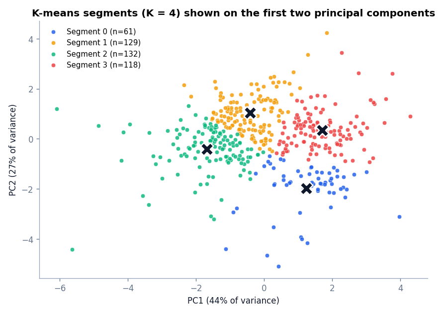
The plot shows segments that form regions of a continuous cloud and not separate islands. That agrees with the silhouette scores. The two plotted components capture a large share of the variance, but a two-dimensional picture of six-dimensional data cannot show every boundary, so some overlap in the plot may be an artifact of the projection.

Interpreting the Segments

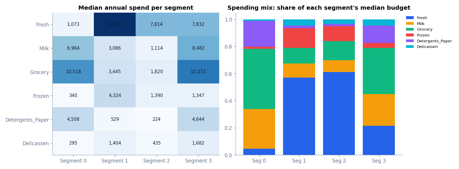
Using the median spend table from the output, here is a plain-language description of each segment. The names are working labels, not facts about the customers.

• Segment 0, “Household and dairy-heavy buyers” (61 customers). Very low Fresh spend (median 1,073) but high Milk (6,964), Grocery (10,518), and Detergents_Paper (4,508). Mostly Retail. These look like stores that sell packaged and household goods and buy little fresh food from this distributor.
• Segment 1, “Fresh and frozen food service” (129). The highest Fresh spend (17,023) and the highest Frozen spend (4,324), with modest Milk, Grocery, and low Detergents_Paper. Almost all Horeca. These are likely restaurants and caterers that depend on fresh and frozen ingredients.
• Segment 2, “Small food-service accounts” (132). Moderate Fresh (7,814) and low spending in every other category, including the lowest Milk, Grocery, and Detergents_Paper. Almost all Horeca. These are low-volume customers across the board.
• Segment 3, “Large mixed retail buyers” (118). The highest Milk (8,482), Grocery (12,272), and Delicassen (1,682) with moderate Fresh (7,832) and high Detergents_Paper (4,644). Mostly Retail. These are broad buyers with strong volume in packaged goods.

Actionable Conclusions

The point of segmentation is to change what the business does. These suggestions follow from the segment profiles, and each should be tested before it is rolled out widely.

• Segment 1: prioritize delivery frequency and freshness. Offer bundles that combine fresh and frozen products. Because Fresh is their main spend, late or poor-quality deliveries would hurt most.
• Segment 3: negotiate volume discounts on grocery, dairy, and household categories, and cross-sell delicatessen items, where their spending is highest.
• Segment 0: they buy packaged and household goods but almost no fresh items. Test whether a small fresh range is of interest, or focus on reliable supply of the categories they already buy.
• Segment 2: serve at low cost. Consider self-service ordering, standard delivery windows, and promotions aimed at increasing basket size, because each account is small.
• Measure the effect. Track revenue, order frequency, and retention per segment before and after any change, ideally with a control group, since a segment is a description and not proof that a tactic works.

Limitations and Next Steps

• Weak cluster separation. The silhouette scores below 0.3 show overlapping groups. Treat segment membership as approximate, especially for customers near the boundary. A Gaussian mixture model would give membership probabilities for exactly those customers.
• K was chosen by judgment. Different reasonable analysts could choose K = 2, 3, or 5. Document the choice and test its stability by re-running with different seeds and by bootstrapping the data.
• One snapshot, six features. The data holds annual spending only. Real segmentation would add recency, order frequency, margins, and tenure.
• Preprocessing changes the answer. Without the log transform, a few very large customers would dominate the clusters. Try both and compare.
• Other algorithms. Compare with hierarchical clustering, or use DBSCAN and anomaly detection to examine the very largest customers separately, because they may need individual account management and not segment-level treatment.
• Dimensionality reduction. With many more features, apply PCA before clustering, or learn a compact representation with an autoencoder.

Common Mistakes in Customer Segmentation

• Clustering on raw, unscaled, skewed spending data.
• Including categorical codes such as region as if they were quantities.
• Choosing K only from a metric, or only to get a tidy number, without checking if the segments can be described.
• Presenting segments as natural categories when the metrics show overlap.
• Profiling segments with means instead of medians on skewed data.
• Stopping at the plot and never turning the segments into actions that can be tested.

Frequently Asked Questions

Which algorithm is best for customer segmentation?

K-means is the usual starting point because it is fast and easy to explain. Hierarchical clustering helps when you want to explore different numbers of segments, and Gaussian mixtures help when you need soft membership.

How many customer segments should I create?

Use metrics such as silhouette and inertia to narrow the range, then choose the number that gives distinct, stable, and actionable segments. Three to six is common in practice.

Why do you use the log transform?

Customer spending is heavily right-skewed. The log transform reduces the influence of a few very large customers so that centroids reflect typical behavior.

Can I use this approach on my own customer data?

Yes. Replace the loading step and the spend_cols list with your behavioral features, and repeat the transformation, scaling, model selection, and profiling steps.

Is the dataset suitable for production decisions?

It is a small educational dataset from a single distributor. Use it to learn the workflow, and validate any business conclusion with your own current data.

Conclusion

This project took raw customer spending through the full unsupervised learning workflow: inspect and transform the data, scale it, test several values of K, fit K-means, evaluate with internal metrics and an outside reference, visualize with PCA, and translate the result into segment descriptions and actions. The most important lesson is honest interpretation. The metrics said the groups overlap, and the segments are still useful because they are distinguishable, reasonably sized, and linked to different business actions.

This completes the BeingNeuron unsupervised learning series. If you want to revisit the foundations, start again from What Is Unsupervised Learning?, or compare clustering methods on this dataset by rerunning the script with hierarchical clustering.

References

• Cardoso, M. G. M. S. Wholesale customers dataset. UCI Machine Learning Repository: archive.ics.uci.edu/dataset/292/wholesale+customers
• scikit-learn documentation: K-means
• scikit-learn documentation: davies_bouldin_score
• pandas documentation