Anomaly Detection in Machine Learning: Finding Outliers in Unlabeled Data

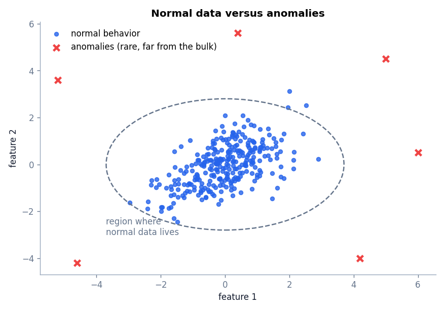
Anomaly detection in machine learning is the task of finding data points that do not fit the pattern of the rest of the data. These points are called anomalies or outliers. They matter because they often represent the events people care about most: a fraudulent payment, a failing machine, a network intrusion, or a data entry error.

In most real projects there are almost no labeled examples of anomalies, so unsupervised methods are the practical starting point. This article explains what anomalies are, how the two most popular unsupervised detectors, Isolation Forest and Local Outlier Factor, work, how to run them in Python, and why evaluating anomaly detectors is harder than it looks.

What Are Anomalies and Outliers?

An anomaly is an observation that differs so much from the normal pattern that it seems to come from a different process. The words anomaly and outlier are often used interchangeably, although some authors reserve “outlier” for extreme values caused by noise and “anomaly” for points of real interest.

Types of anomalies

• Point anomalies: a single observation that is unusual on its own, such as a transaction ten times larger than any previous one.
• Contextual anomalies: a value that is normal in general but unusual in its context. A temperature of 30 degrees Celsius is normal in July and alarming in January.
• Collective anomalies: a group of observations that is unusual together even if each individual value looks normal, such as a flat line in a heart-rate signal.

This article focuses on point anomalies in tabular numeric data, the most common beginner case.

Unsupervised, Semi-Supervised, and Supervised Detection

• Supervised: you have labeled normal and anomalous examples and train a classifier. This is rare, and anomalies are so scarce that the classes are extremely imbalanced.
• Semi-supervised (novelty detection): you train only on data you believe is normal, then flag anything that differs from it. Autoencoders, covered in the next article, are often used this way.
• Unsupervised (outlier detection): you have one unlabeled dataset that may contain anomalies, and the algorithm decides which points are unusual. Isolation Forest and Local Outlier Factor are used this way.

The unsupervised setting rests on two assumptions: anomalies are rare, and they are different from normal points.

Isolation Forest

The idea

Most detectors first learn what normal looks like and then measure distance from it. Isolation Forest takes a different route. It asks how easy it is to isolate each point.

Imagine picking a random feature and a random split value between that feature’s minimum and maximum, over and over, cutting the data into smaller and smaller boxes until one point is alone in its box. A point far from the crowd gets isolated after very few cuts. A point inside a dense region needs many cuts, because there are many neighbors to separate it from.

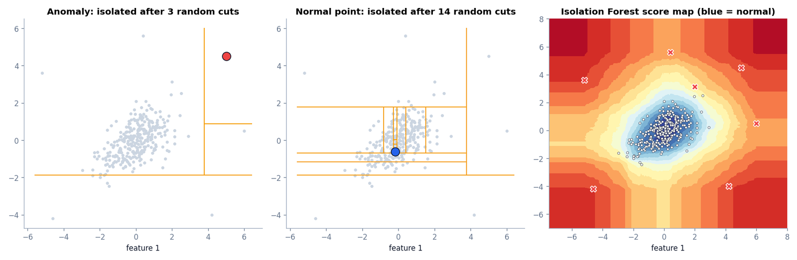
The first two panels show one random draw of cuts. The anomaly was isolated after three cuts and the normal point after fourteen. A single random sequence can be lucky or unlucky, so the algorithm builds many random trees, called isolation trees, and averages the path length across all of them.

The anomaly score

Let h(x) be the number of splits needed to isolate x in a tree, and E[h(x)] its average over the forest. The anomaly score is

s(x, n) = 2^{−E[h(x)] / c(n)}

where c(n) is the average path length of an unsuccessful search in a binary search tree built from n points, used to normalize the score. Scores close to 1 indicate anomalies, scores well below 0.5 indicate normal points, and scores near 0.5 everywhere suggest no clear anomalies. Note that scikit-learn’s score_samples returns the negative of this score, so lower values are more anomalous.

Strengths and weaknesses

• Fast, with linear time in the number of points, and works on large datasets.
• No distance calculations between points, so it is less affected by scale and handles many features.
• Needs few parameters: the number of trees and the expected contamination.
• Weaker at local anomalies near dense clusters and with high-dimensional data in which most features are irrelevant.

Local Outlier Factor (LOF)

The idea

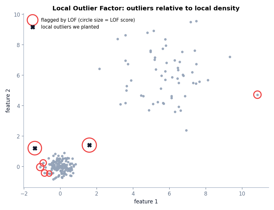
Consider data with a very dense cluster and a very sparse cluster. A point that is 2 units away from its neighbors is a clear outlier in the dense cluster but completely normal in the sparse one. A single global distance threshold cannot handle both. LOF compares each point’s local density with the density of its neighbors.

How LOF is computed

1. For each point p, find its k nearest neighbors.
2. Compute the reachability distance from p to a neighbor o: reach-dist_k(p, o) = max( k-distance(o), d(p, o) ). This smooths out very small distances.
3. Compute the local reachability density, the inverse of the average reachability distance from p to its neighbors: lrd_k(p) = 1 / ( mean reach-dist_k(p, o) ).
4. Compute the LOF score as the average ratio of the neighbors’ density to p’s density:

LOF_k(p) = ( Σ_{o ∈ Nk(p)} lrd_k(o) / lrd_k(p) ) / |N_k(p)|

A score near 1 means p has about the same density as its neighbors. A score well above 1 means p lies in a much sparser area than its neighbors, which marks it as a local outlier.

Strengths and weaknesses

• Detects local anomalies in data with clusters of different density.
• The score has an intuitive interpretation relative to 1.
• Needs distance computations, so it is slower on large data, and scale matters.
• Results depend on the choice of k. Too small a value is noisy, and too large a value blurs local structure.
• By default, scikit-learn’s LocalOutlierFactor scores only the data it was fitted on. To score new points, create it with novelty=True and fit on data assumed to be normal.

Anomaly Detection in Python

The script below plants six obvious outliers in a cloud of 300 normal points and runs Isolation Forest. It then builds a second dataset with a dense and a sparse cluster, plants two local outliers, and runs LOF. The planted labels are used only at the end to check the results. Neither algorithm sees them. You need numpy and scikit-learn.

import numpy as np
from sklearn.ensemble import IsolationForest
from sklearn.neighbors import LocalOutlierFactor

rng = np.random.default_rng(42)
normal = rng.normal(0, 1, (300, 2)) @ np.array([[1.0, 0.4], [0.0, 0.8]])
planted = np.array([[5.0, 4.5], [-5.2, 3.6], [4.2, -4.0], [-4.6, -4.2], [6.0, 0.5], [0.4, 5.6]])
X = np.vstack([normal, planted])
is_planted = np.r_[np.zeros(len(normal), bool), np.ones(len(planted), bool)]  # used ONLY to check results

# Isolation Forest
iso = IsolationForest(n_estimators=200, contamination=0.02, random_state=42).fit(X)
iso_flag = iso.predict(X) == -1            # -1 means anomaly
scores = iso.score_samples(X)              # lower = more anomalous
print("Isolation Forest flagged:", int(iso_flag.sum()), "points")
print("Planted outliers caught:", int((iso_flag & is_planted).sum()), "of", int(is_planted.sum()))
print("False positives:", int((iso_flag & ~is_planted).sum()))
print("Lowest 3 scores:", np.round(np.sort(scores)[:3], 3))

# Local Outlier Factor on data with two different densities
dense = rng.normal([0, 0], 0.35, (150, 2))
sparse = rng.normal([6, 6], 1.5, (60, 2))
local_out = np.array([[1.6, 1.4], [-1.4, 1.2]])
Y = np.vstack([dense, sparse, local_out])
lof = LocalOutlierFactor(n_neighbors=20, contamination=0.03)
flag = lof.fit_predict(Y) == -1
factor = -lof.negative_outlier_factor_      # about 1 = normal, much larger = outlier
print("\nLOF flagged:", int(flag.sum()), "points")
print("Planted local outliers flagged:", flag[-2:].tolist(), "with LOF scores", np.round(factor[-2:], 2).tolist())
print("Median LOF score of all points:", round(float(np.median(factor)), 2))

Isolation Forest flagged: 7 points
Planted outliers caught: 6 of 6
False positives: 1
Lowest 3 scores: [-0.786 -0.785 -0.771]

LOF flagged: 7 points
Planted local outliers flagged: [True, True] with LOF scores [4.36, 4.18]
Median LOF score of all points: 1.06

What the code and output show:

• contamination=0.02 tells Isolation Forest to flag the 2 percent of points with the lowest scores. It flagged 7 points: all 6 planted outliers and 1 normal point. That one false positive is the price of forcing a fixed flag rate.
• predict returns −1 for anomalies and 1 for normal points. The lowest score_samples values are about −0.79, the most anomalous in the dataset.
• LOF with n_neighbors=20 flagged 7 points, including both planted local outliers, with LOF scores of 4.36 and 4.18. The median score across all points is 1.06, close to 1 as expected for typical points.
• negative_outlier_factor_ stores the negative of the LOF score, which is why the script negates it to read a value where larger means more anomalous.

Other Unsupervised Approaches

• DBSCAN noise points. Points that belong to no dense region are labeled noise. See DBSCAN Clustering Explained.
• Gaussian mixture density. Points with very low likelihood under a fitted mixture are unusual. See Gaussian Mixture Models.
• PCA reconstruction error. Points that the principal components reconstruct poorly deviate from the main structure. See PCA Explained.
• Autoencoder reconstruction error. The neural network version of the same idea, covered in the next article.
• One-class SVM and robust covariance (Elliptic Envelope). Boundary-based methods that are also available in scikit-learn.

Practical Applications

• Finance: flagging unusual transactions for review.
• Manufacturing and maintenance: detecting sensor readings that precede equipment failure.
• Cybersecurity: spotting abnormal network traffic or login patterns.
• Healthcare data quality: finding implausible measurements and recording errors.
• Data cleaning: locating suspicious rows before model training.
• Operations monitoring: alerting on unusual traffic or latency patterns.

A Practical Workflow for an Anomaly Detection Project

1. Define what “anomalous” means for the business and what an alert will trigger.
2. Choose features that could reveal the anomaly, and scale them when the method needs it.
3. Start with a simple baseline, such as Isolation Forest with default settings.
4. Rank points by score and have a domain expert review the top results. Their feedback is your first set of labels.
5. Use those labels to evaluate with precision at the top of the ranking, and to choose a threshold.
6. Monitor the alert rate over time and refit when the data drifts.

Evaluation Challenges

Evaluating an anomaly detector is difficult, and many tutorials gloss over it.

• No ground truth. In a truly unsupervised project you do not know which points are anomalies. Any accuracy number depends on labels that you often cannot get.
• Extreme class imbalance. If 0.1 percent of the data is anomalous, a detector that flags nothing is 99.9 percent accurate. Use precision, recall, and the precision-recall curve instead of accuracy. ROC AUC can look flattering on imbalanced data.
• The contamination parameter is a guess. Setting contamination makes the detector flag a fixed percentage regardless of whether that many anomalies exist.
• Cost asymmetry. A missed fraud case and a wrongly flagged customer have different costs. Choose thresholds with those costs in mind.
• Synthetic benchmarks mislead. Planted outliers, as in the example above, are easier to find than real ones. The 6 of 6 result shows that the code works, not that real-world detection will be this clean.
• Drift. What counts as normal changes over time, so a detector needs monitoring and periodic refitting.

False Positives and Limitations

• False positives are inevitable. Unusual does not mean bad. A rare but legitimate customer purchase can be flagged. Review capacity limits how many alerts are useful, so rank by score and tune the threshold to what analysts can handle.
• Rare does not mean important. The algorithm finds statistical oddities. A person decides whether they matter.
• Feature choice dominates. If the anomaly is invisible in the chosen features, no algorithm can find it.
• Scale and preprocessing. Distance-based methods such as LOF need standardized features. Isolation Forest is less sensitive but still depends on informative features.
• Masking and swamping. A cluster of anomalies can look like a small normal group and hide each other, and normal points near anomalies can be dragged into a flagged region.
• Explanations are limited. A score says that a point is unusual, not why. Add feature-level analysis if people must act on the alert.

Common Mistakes

• Reporting accuracy on imbalanced anomaly data.
• Setting contamination without a reason, and treating the flagged count as a finding.
• Not scaling features before LOF.
• Training on data that already contains many anomalies when using a novelty-detection method.
• Presenting flagged points as confirmed fraud or faults instead of candidates for review.

Frequently Asked Questions

What is the difference between an anomaly and an outlier?

In practice, the terms are used interchangeably. Some authors call extreme values caused by errors “outliers” and meaningful rare events “anomalies”.

Is anomaly detection supervised or unsupervised?

It can be either. Unsupervised methods such as Isolation Forest and LOF need no labels. Supervised methods need labeled anomalies, which are usually scarce.

How does Isolation Forest work?

It builds many random trees that split the data at random thresholds. Anomalies are isolated in fewer splits, so they have shorter average path lengths and higher anomaly scores.

When should I use LOF instead of Isolation Forest?

Use LOF when your data contains clusters of different density and you care about local outliers. Use Isolation Forest for larger datasets, higher dimensions, or when you need speed.

How do I choose the contamination value?

Use a domain estimate of how common anomalies are, or flag by score ranking and let reviewers decide how deep to go. Avoid treating contamination as a measured quantity.

Conclusion

Anomaly detection finds the points that the rest of the data does not explain. Isolation Forest isolates points with random cuts and works well on large datasets. Local Outlier Factor compares each point’s density with its neighbors and catches local outliers. Both work without labels, and both produce candidates that need human judgment. The hardest part is not running the algorithm but evaluating it honestly and handling false positives.

Neural networks offer another route: train a model to rebuild normal data and flag whatever it fails to rebuild. Continue with Autoencoders Explained: How Neural Networks Learn Without Labels.

References

• scikit-learn documentation: Novelty and outlier detection
• Liu, F. T., Ting, K. M., and Zhou, Z.-H. (2008). Isolation Forest. Proceedings of the IEEE International Conference on Data Mining.
• Breunig, M. M., Kriegel, H.-P., Ng, R. T., and Sander, J. (2000). LOF: Identifying density-based local outliers. Proceedings of ACM SIGMOD.