Hierarchical Clustering Explained: Agglomerative Clustering and Dendrograms

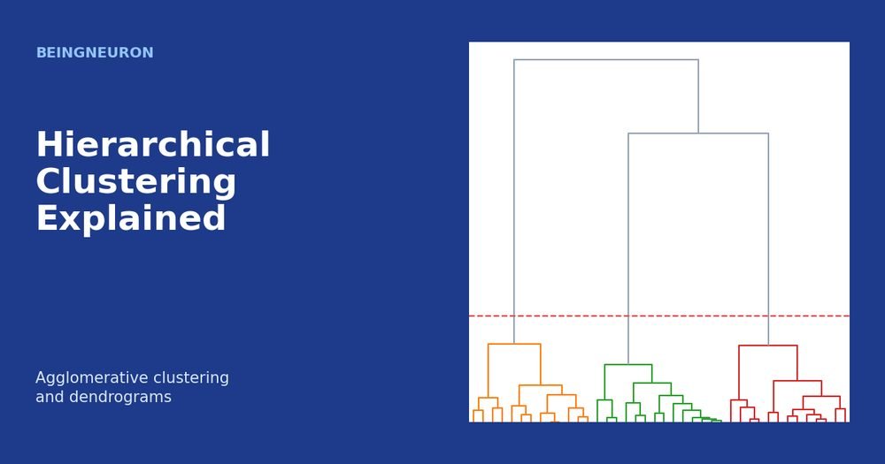
Hierarchical clustering builds a tree of clusters instead of a single flat partition. At the bottom of the tree every data point is its own cluster. At the top, all points form one cluster. Every level in between is a valid grouping, so you can look at the data at any level of detail without rerunning the algorithm.

This article explains the two approaches, agglomerative and divisive clustering, shows how to read a dendrogram, compares the main linkage methods, and implements everything in Python with SciPy and scikit-learn. It also compares hierarchical clustering with K-means, which you may know from the previous article.

What Is Hierarchical Clustering?

Hierarchical clustering is an unsupervised method that arranges data into nested clusters. Unlike K-means, it does not ask you to choose the number of clusters before you start. You build the whole hierarchy first and decide how many clusters you want afterward by cutting the tree at a chosen height.

This makes it useful for exploration. If you do not know whether your data has two, five, or twelve natural groups, the tree shows you how clusters join as the distance threshold grows.

Agglomerative vs Divisive Clustering

Agglomerative (bottom-up)

Agglomerative clustering starts with n clusters, one per point. At every step it merges the two closest clusters. After n − 1 merges only one cluster remains. This is the version used almost everywhere in practice, including scikit-learn’s AgglomerativeClustering and SciPy’s linkage.

Divisive (top-down)

Divisive clustering starts with all points in one cluster and repeatedly splits a cluster into two. Finding the best split is expensive, because there are exponentially many ways to divide a set of points, so divisive methods rely on heuristics such as running K-means with K = 2 at each step. They are rare in everyday projects, and the rest of this article focuses on the agglomerative approach.

How Agglomerative Clustering Works Step by Step

1. Treat each point as a cluster of size one.
2. Compute the distance between every pair of clusters.
3. Merge the two clusters with the smallest distance.
4. Update the distances between the new cluster and all others using the chosen linkage rule.
5. Repeat steps 3 and 4 until one cluster remains.

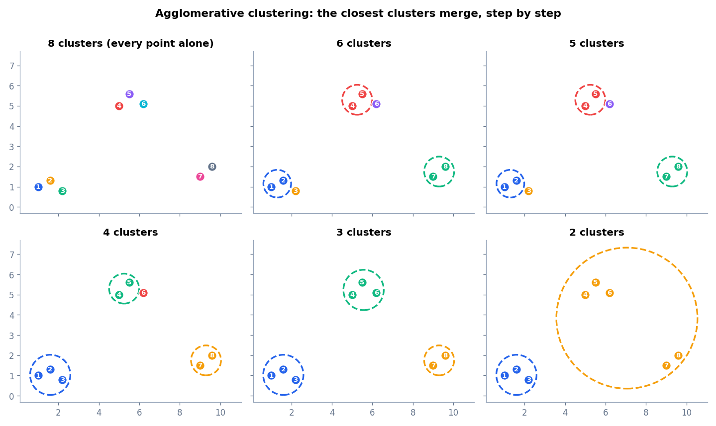
The figure shows eight points. Points 1, 2, and 3 sit close together, as do 4, 5, and 6, and 7 and 8. Those tight groups merge first. With three clusters left, the algorithm must decide which of the remaining groups are closest, and the answer depends on the linkage method.

Reading a Dendrogram

A dendrogram is a tree diagram that records every merge.

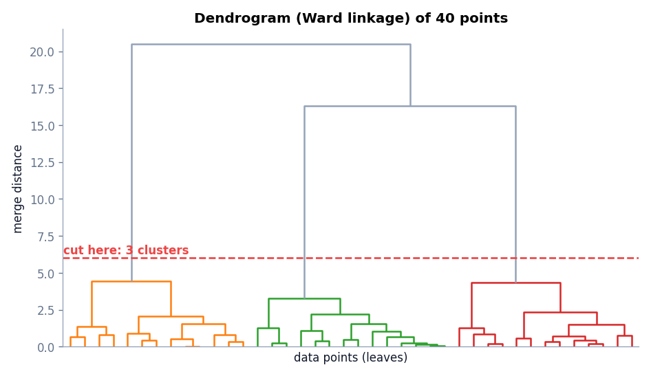
• The leaves along the bottom are the data points.
• Each U-shaped link is a merge between two clusters.
• The height of a link is the distance between the two clusters when they merged.
• Long vertical lines show that clusters were far apart when they joined, which signals a natural boundary between groups.

To get a flat clustering, draw a horizontal line across the dendrogram. Every branch that the line crosses becomes one cluster. In the figure, the red line at a height of 6 crosses three branches, so the data splits into three clusters. A practical rule is to cut where the vertical gaps between merge heights are largest, because that is where the algorithm had to jump across a large distance to combine groups.

Note that the leaf order along the bottom has no meaning. The two children of every merge can be swapped without changing the tree. Only vertical heights and the grouping structure are meaningful.

A Worked Example With Five Numbers

Take five one-dimensional points: 1, 2, 6, 7, and 15. At the start every point is its own cluster. The closest pairs are (1, 2) and (6, 7), each at distance 1, so both pairs merge first under any linkage method. Now the methods disagree about what comes next.

• Single linkage measures the closest members. The distance between {1, 2} and {6, 7} is |2 − 6| = 4, and the distance from {6, 7} to 15 is |15 − 7| = 8. The clusters merge at heights 1, 1, 4, and then 8, when the point 15 joins.
• Complete linkage measures the farthest members. The distance between {1, 2} and {6, 7} is |1 − 7| = 6, and the final merge with 15 happens at |1 − 15| = 14. The heights are 1, 1, 6, and 14.

The merge order is the same here, but the heights differ, and on messier data the order itself can change. Heights matter because the dendrogram cut depends on them.

Linkage Methods

After a merge, the algorithm needs the distance between the new cluster and every other cluster. A linkage method defines how to measure the distance between two clusters A and B. Let d(a, b) be the distance between two individual points.

Single linkage

D(A, B) = min d(a, b)

The distance is that of the closest pair of points, one from each cluster. Single linkage can follow long chains of nearby points, so it finds elongated or curved clusters, but it is easily fooled by noise points that form a bridge between two groups. This is called the chaining effect.

Complete linkage

D(A, B) = max d(a, b)

The distance is that of the farthest pair of points. It prefers compact clusters with similar diameters, but one outlier can delay a merge.

Average linkage

D(A, B) = (1 / |A||B|) Σ_a∈A Σ_b∈B d(a, b)

The distance is the mean over all pairs. It is a compromise between single and complete linkage and is less sensitive to outliers than complete linkage.

Ward linkage

Ward linkage merges the pair of clusters whose union causes the smallest increase in total within-cluster variance. It is the hierarchical counterpart of K-means and its objective of compact clusters. It requires Euclidean distance, and it tends to produce clusters of similar size. Ward is the default in scikit-learn and a good first choice for numeric data.

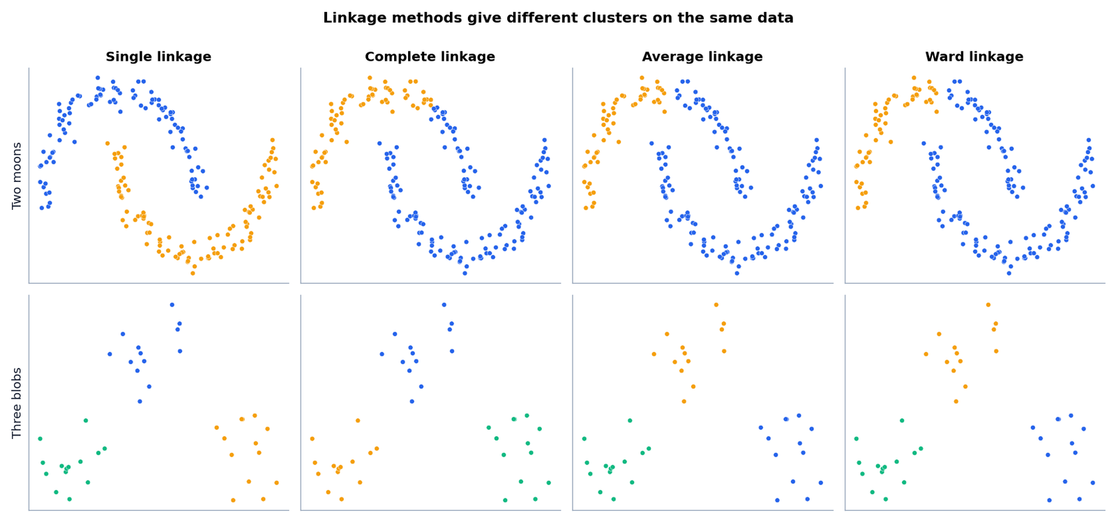
The comparison shows why the choice matters. On three compact blobs, all four methods agree. On two crescent shapes, single linkage follows each curve and recovers both groups, while complete, average, and Ward linkage prefer compact pieces and split the data in other ways. No linkage method is best for every dataset.

Distance Measures

Linkage works on top of a point-to-point distance measure. Euclidean distance is the default and the only choice for Ward linkage. Manhattan distance can be used with single, complete, and average linkage, and cosine distance is common for text vectors. See the previous overview article for the formulas. As with every distance-based method, scale your features first.

Hierarchical Clustering in Python

The script below creates 40 points from three groups, standardizes them, builds the linkage tree with SciPy, draws the dendrogram, and then extracts three clusters in two ways. It ends by comparing linkage methods on a two-crescent dataset. You need numpy, scipy, matplotlib, and scikit-learn.

import numpy as np
import matplotlib.pyplot as plt
from sklearn.datasets import make_blobs
from sklearn.preprocessing import StandardScaler
from sklearn.cluster import AgglomerativeClustering
from sklearn.metrics import silhouette_score
from scipy.cluster.hierarchy import linkage, dendrogram, fcluster

X, _ = make_blobs(n_samples=40, centers=[(-3, 0), (0, 3.5), (3, 0)], cluster_std=0.7, random_state=3)
X = StandardScaler().fit_transform(X)

# Build the full merge tree with Ward linkage.
Z = linkage(X, method="ward")
print("Linkage matrix shape:", Z.shape, "(one row per merge)")
print("Last three merge heights:", np.round(Z[-3:, 2], 2))

# Draw the dendrogram.
plt.figure(figsize=(9, 4))
dendrogram(Z, no_labels=True)
plt.title("Ward linkage dendrogram")
plt.ylabel("Merge distance")
plt.show()

# Cut the tree into 3 clusters with SciPy...
labels_scipy = fcluster(Z, t=3, criterion="maxclust")
# ...or fit the same model directly with scikit-learn.
agg = AgglomerativeClustering(n_clusters=3, linkage="ward")
labels_sk = agg.fit_predict(X)
print("Cluster sizes (SciPy):", np.bincount(labels_scipy)[1:])
print("Cluster sizes (scikit-learn):", np.bincount(labels_sk))
print("Silhouette:", round(silhouette_score(X, labels_sk), 3))

# Linkage matters when clusters are not compact blobs. Try two crescent shapes.
from sklearn.datasets import make_moons
moons, _ = make_moons(n_samples=200, noise=0.07, random_state=1)
print("\nLinkage comparison on two moons (cluster sizes):")
for method in ["single", "complete", "average", "ward"]:
    lab = AgglomerativeClustering(n_clusters=2, linkage=method).fit_predict(moons)
    print(f"{method:9s} sizes = {np.bincount(lab)}")

Linkage matrix shape: (39, 4) (one row per merge)
Last three merge heights: [2.46 7.96 8.69]
Cluster sizes (SciPy): [14 13 13]
Cluster sizes (scikit-learn): [13 14 13]
Silhouette: 0.685

Linkage comparison on two moons (cluster sizes):
single    sizes = [100 100]
complete  sizes = [133  67]
average   sizes = [146  54]
ward      sizes = [146  54]

What the code does:

• linkage(X, method="ward") returns a matrix with one row per merge. Each row stores the two merged cluster indices, the merge distance, and the size of the new cluster. With 40 points there are 39 merges, which matches the printed shape.
• The last three merge heights (2.46, 7.96, 8.69) show the large jump before the final merges. The tree has three clear groups: the final two merges happen at much larger distances than the earlier ones.
• fcluster(Z, t=3, criterion="maxclust") cuts the tree to give exactly three clusters. SciPy numbers clusters from 1, so the script drops the unused index 0 when counting.
• AgglomerativeClustering(n_clusters=3, linkage="ward") returns the same grouping. Cluster numbers can be permuted between libraries, which explains why the size lists look reordered.
• The silhouette score of 0.685 confirms compact, separated groups.
• The final loop shows the effect of linkage on crescents. Single linkage returns two clusters of 100 points each, which is the true structure. Complete linkage gives 133 and 67, and average and Ward give 146 and 54.

The dendrogram image in this article was drawn from the unscaled coordinates, so its heights differ from the standardized heights printed by the script. The shape of the tree is the same.

Choosing the number of clusters

• Look for the largest vertical gap in the dendrogram and cut inside it.
• Compute silhouette scores for several cuts and compare them.
• Inspect the cluster profiles and keep the number of groups that you can interpret and act on.

Practical tips for real projects

Start with Ward linkage and Euclidean distance on standardized features, then plot the dendrogram and look at the largest vertical gaps. If the tree looks like one long chain, switch from single to average or Ward linkage. If the dataset has more than a few thousand rows, sample it or cluster the centroids of a fast first-pass K-means run. Always compute the cophenetic correlation, available as scipy.cluster.hierarchy.cophenet, when you want a number that tells you how faithfully the tree preserves the original pairwise distances.

Hierarchical Clustering vs K-Means

Aspect	Hierarchical clustering	K-means
Number of clusters	Chosen after building the tree	Chosen before running
Output	Full hierarchy and dendrogram	Flat partition and centroids
Determinism	Deterministic for a given setup	Depends on initialization
Cluster shapes	Depends on linkage	Round, similar size
Scalability	Memory and time grow quickly with n	Linear in n
Predicting new points	No built-in method	Yes, nearest centroid

Use K-means for large datasets and when you want centroids for prediction. Use hierarchical clustering when the dataset is small or medium, when you want to explore the structure at several levels, or when a tree is itself the result you need, as in gene expression studies and taxonomy building.

Advantages of Hierarchical Clustering

• No need to fix the number of clusters before running the algorithm.
• The dendrogram shows relationships between clusters, not only membership.
• The result is deterministic, so there are no random restarts.
• Several linkage methods adapt it to different cluster shapes.

Limitations

• Poor scalability. The algorithm needs the pairwise distance matrix, which grows with n², and the time cost is at least O(n²). Datasets with tens of thousands of points become slow or memory-heavy.
• Merges are permanent. Once two clusters merge, the algorithm never reconsiders that decision, so an early mistake spreads.
• Sensitive to noise and outliers, especially with single linkage (chaining) and complete linkage (one extreme point).
• Sensitive to scale and metric. Unscaled features give distorted trees.
• Dendrograms get unreadable with hundreds of leaves. Truncate the plot or use the truncate_mode option in SciPy.

Common Mistakes

• Using Ward linkage with a non-Euclidean distance. Ward assumes Euclidean geometry.
• Reading the order of leaves as a similarity ranking.
• Forgetting to standardize features.
• Using single linkage on noisy data and wondering why one giant cluster appears.
• Cutting the dendrogram at an arbitrary height without checking the clusters.

Frequently Asked Questions

What is the difference between agglomerative and divisive clustering?

Agglomerative clustering starts with single points and merges upward. Divisive clustering starts with one cluster and splits downward. Agglomerative is far more common.

Which linkage method should I use?

Start with Ward for numeric, compact clusters. Try average linkage as a robust alternative and single linkage when you expect elongated shapes and have little noise.

How do I choose the number of clusters from a dendrogram?

Cut the tree where the vertical distance between consecutive merges is large. Confirm the choice with silhouette scores and by inspecting the clusters.

Can hierarchical clustering handle large datasets?

Not well. For very large data, use K-means, mini-batch K-means, or DBSCAN, or run hierarchical clustering on a sample or on cluster centroids.

Does hierarchical clustering need labels?

No. It is unsupervised and uses only the features.

Conclusion

Hierarchical clustering gives you the whole family tree of your data. Agglomerative methods merge the closest clusters repeatedly, the dendrogram records the merge distances, and the linkage rule decides what “closest” means for groups of points. It is excellent for small and medium datasets and exploratory analysis, and weaker on large or noisy data.

Both K-means and hierarchical clustering struggle when clusters have irregular shapes or when noise is present. The next article introduces an algorithm designed for exactly that situation: DBSCAN Clustering Explained: Core Points, Noise, and Outliers.

References

• SciPy documentation: Hierarchical clustering (scipy.cluster.hierarchy)
• scikit-learn documentation: Hierarchical clustering
• Ward, J. H. (1963). Hierarchical grouping to optimize an objective function. Journal of the American Statistical Association, 58(301), 236 to 244.