Principal Component Analysis (PCA) Explained with Python

Principal Component Analysis (PCA) is a dimensionality reduction method that rewrites a dataset using a smaller number of new features, called principal components, while keeping as much of the original variation as possible. It is one of the oldest and most widely used tools in machine learning, and it is the standard first step when a dataset has too many columns to inspect, plot, or model comfortably.

The earlier articles in this series grouped rows of data with K-means, hierarchical clustering, and DBSCAN. PCA works on the columns instead. This guide explains the idea with a simple picture, introduces variance, covariance, eigenvectors, and eigenvalues at a practical level, builds PCA from scratch in NumPy, and then applies scikit-learn to a 64-feature image dataset.

What Is Dimensionality Reduction?

The dimensions of a dataset are its features. A table with 64 columns lives in 64-dimensional space. High dimensionality causes practical problems:

• You cannot plot more than three dimensions directly.
• Models need more data, more memory, and more time as features increase.
• Distances become less informative in high dimensions, which hurts clustering and nearest-neighbor methods.
• Many features are correlated, so they repeat the same information.

Dimensionality reduction addresses these problems by finding a smaller set of features that still describes the data well. PCA does this with linear combinations of the original features.

The Intuition Behind PCA

Imagine measuring the height and the arm span of 200 adults. The two numbers are strongly related, so the points form a thin diagonal cloud. You do not need both numbers to describe a person. A single number along the diagonal tells you almost everything, and the small distance from the diagonal is minor detail.

PCA finds that diagonal automatically. It looks for the direction along which the data varies most, calls it the first principal component, and then looks for the next most varying direction that is perpendicular to the first, and so on.

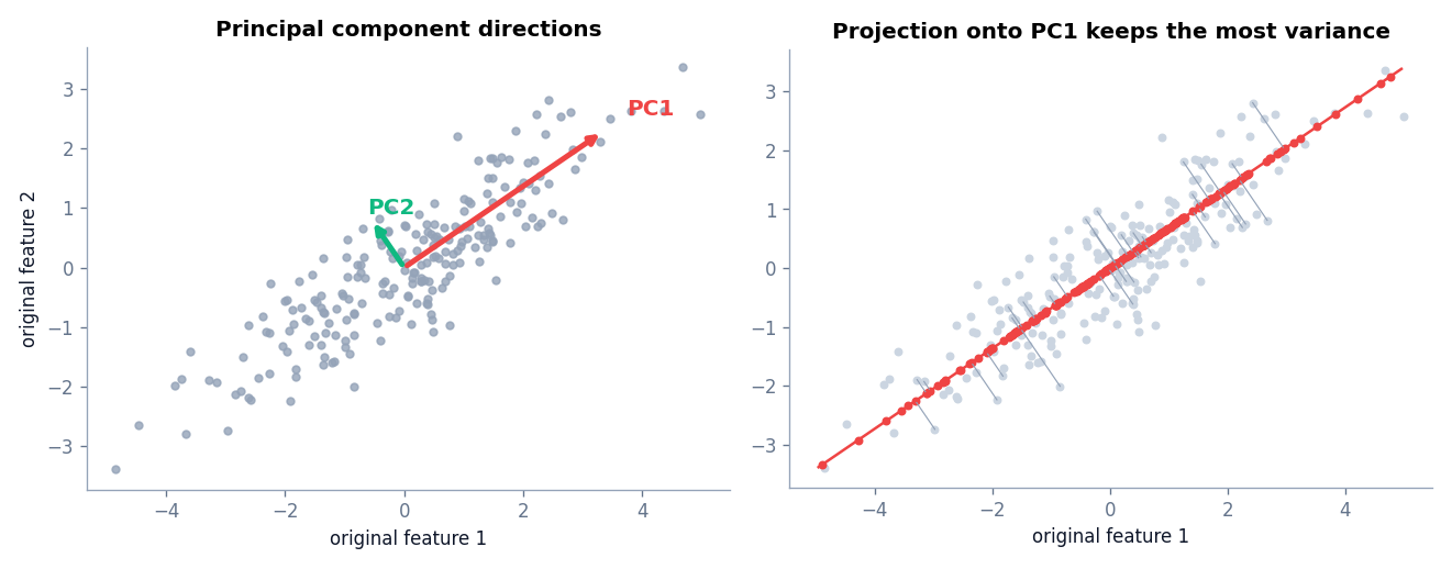
In the left panel, PC1 points along the long axis of the cloud and PC2 is perpendicular to it with a much smaller spread. In the right panel, every point is projected onto the PC1 line. The two-dimensional cloud becomes a one-dimensional set of positions, and most of the spread is preserved.

The Math Behind PCA, Step by Step

Variance and covariance

Variance measures how spread out a feature is. Covariance measures how two features vary together: it is positive when they rise and fall together and near zero when they are unrelated. For centered data, the covariance of features j and k is

Cov(x_j, x_k) = (1 / (n − 1)) Σ_i x_ij x_ik

Putting all variances and covariances into a table gives the covariance matrix C, with one row and one column per feature. Its diagonal holds the variances.

Eigenvectors and eigenvalues

An eigenvector of a matrix C is a direction that C only stretches, never rotates. The stretch factor is the eigenvalue:

C v = λ v

For a covariance matrix, eigenvectors are the principal component directions, and each eigenvalue is the variance of the data along its direction. Large eigenvalue means a direction with a lot of variation. Because C is symmetric, its eigenvectors are perpendicular to each other.

The PCA procedure

1. Standardize the features when they use different units or scales.
2. Center the data by subtracting each feature’s mean.
3. Compute the covariance matrix.
4. Compute eigenvectors and eigenvalues and sort them from largest eigenvalue to smallest.
5. Select the top k eigenvectors and stack them into a matrix W of shape (features, k).
6. Project the data: Z = X_centered W. The result Z has k columns, the principal component scores.

The explained variance ratio of component i is its eigenvalue divided by the sum of all eigenvalues:

ratio_i = λ_i / Σ_j λ_j

It tells you what share of the total variance that component carries.

PCA from scratch in NumPy

The script below follows those steps on correlated two-dimensional data and then checks the result against scikit-learn.

import numpy as np
from sklearn.decomposition import PCA

rng = np.random.default_rng(5)
# Correlated 2D data: feature 2 mostly follows feature 1.
X = rng.multivariate_normal([0, 0], [[3.2, 2.0], [2.0, 1.6]], size=220)

# 1. Center the data (subtract each column's mean).
X_centered = X - X.mean(axis=0)

# 2. Covariance matrix of the features.
cov = np.cov(X_centered, rowvar=False)
print("Covariance matrix:\n", np.round(cov, 3))

# 3. Eigen-decomposition. eigh is for symmetric matrices; it returns eigenvalues in ascending order.
eigenvalues, eigenvectors = np.linalg.eigh(cov)
order = np.argsort(eigenvalues)[::-1]
eigenvalues, eigenvectors = eigenvalues[order], eigenvectors[:, order]
print("\nEigenvalues (variance along each component):", np.round(eigenvalues, 3))
print("Explained variance ratio:", np.round(eigenvalues / eigenvalues.sum(), 3))
print("First principal direction:", np.round(eigenvectors[:, 0], 3))

# 4. Project onto the first component (2D -> 1D), then reconstruct.
Z = X_centered @ eigenvectors[:, :1]
X_back = Z @ eigenvectors[:, :1].T + X.mean(axis=0)
print("\nShape after projection:", Z.shape)
print("Mean squared reconstruction error:", round(float(((X - X_back) ** 2).mean()), 4))

# 5. Check against scikit-learn.
pca = PCA(n_components=2).fit(X)
print("\nscikit-learn explained variance:", np.round(pca.explained_variance_, 3))
print("Same eigenvalues?", np.allclose(pca.explained_variance_, eigenvalues))
print("Same direction (up to sign)?", np.allclose(np.abs(pca.components_[0]), np.abs(eigenvectors[:, 0])))

Covariance matrix:
 [[2.871 1.802]
 [1.802 1.467]]

Eigenvalues (variance along each component): [4.103 0.235]
Explained variance ratio: [0.946 0.054]
First principal direction: [-0.826 -0.564]

Shape after projection: (220, 1)
Mean squared reconstruction error: 0.1169

scikit-learn explained variance: [4.103 0.235]
Same eigenvalues? True
Same direction (up to sign)? True

The eigenvalues are 4.103 and 0.235, so the first component carries 94.6 percent of the variance and the second only 5.4 percent. Keeping one component reduces the data from two columns to one, with a mean squared reconstruction error of about 0.117. The scikit-learn numbers match the manual computation. The first direction can differ by sign between implementations, which is why the script compares absolute values. A flipped sign carries the same information.

Reading the loadings

The eigenvectors are also called loadings. In the two-feature example above, the first principal direction is approximately (−0.826, −0.564). The sign is arbitrary, but the message is clear: PC1 is a weighted sum in which both original features contribute with the same sign, with feature 1 contributing a little more. In plain words, PC1 measures “overall size” of the point. For a centered point (3, 2), its PC1 score is −0.826 × 3 + −0.564 × 2 = −3.61. PC2, the perpendicular direction, measures how much the point deviates from the usual relationship between the two features.

With many features, inspecting which original columns have the largest absolute loadings on a component is the standard way to describe what it represents.

PCA compared with t-SNE and UMAP

t-SNE and UMAP are nonlinear methods built mainly for visualization. They often produce more visually separated groups than PCA, but their distances and cluster sizes are harder to interpret, they cannot be inverted back to the original features, and their results vary with parameters and random seeds. PCA is deterministic, fast, invertible, and works as a preprocessing step. Use PCA first and consider the others only for exploratory plots.

High-Dimensional Data to Two Dimensions

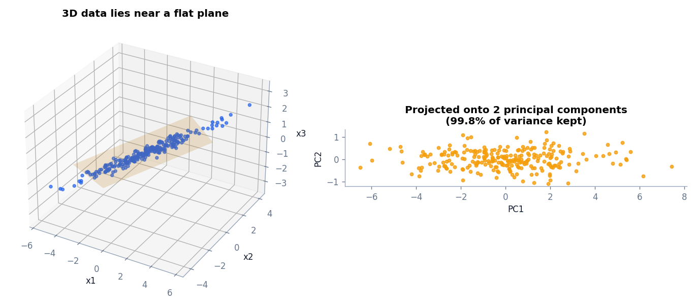
The figure shows the same idea in three dimensions. The points lie close to a flat plane tilted in space. PCA finds that plane and projects the points onto it. Two components keep about 99.8 percent of the variance, so the flattened picture is almost a perfect description of the original data.

PCA in Python With scikit-learn

Real data is rarely so tidy. The scikit-learn digits dataset has 1,797 handwritten digit images, each stored as 64 pixel values (an 8 by 8 grid). The script reduces those 64 features, measures how much variance each component carries, reconstructs the images to see what was lost, and plots a two-dimensional view. The digit labels are used only to color the plot. PCA never receives them.

import numpy as np
import matplotlib.pyplot as plt
from sklearn.datasets import load_digits
from sklearn.decomposition import PCA
from sklearn.preprocessing import StandardScaler

digits = load_digits()
X = digits.data            # 1797 images, 64 pixel features each
print("Original shape:", X.shape)

# Standardize first: PCA is sensitive to feature scale.
X_scaled = StandardScaler().fit_transform(X)

# Fit PCA with all components to inspect explained variance.
pca_full = PCA().fit(X_scaled)
cumulative = np.cumsum(pca_full.explained_variance_ratio_)
print("Variance explained by PC1, PC2:", np.round(pca_full.explained_variance_ratio_[:2], 3))
print("Components needed for 90% variance:", int(np.argmax(cumulative >= 0.90)) + 1)
print("Components needed for 95% variance:", int(np.argmax(cumulative >= 0.95)) + 1)

# Keep enough components for 95% of the variance.
pca95 = PCA(n_components=0.95).fit(X_scaled)
X_reduced = pca95.transform(X_scaled)
print("Reduced shape:", X_reduced.shape)

# Reconstruct and measure what was lost.
X_back = pca95.inverse_transform(X_reduced)
print("Mean squared reconstruction error:", round(float(((X_scaled - X_back) ** 2).mean()), 4))

# 2D projection for plotting. Labels are used ONLY to color the plot.
X_2d = PCA(n_components=2).fit_transform(X_scaled)
plt.scatter(X_2d[:, 0], X_2d[:, 1], c=digits.target, cmap="tab10", s=8)
plt.xlabel("PC1"); plt.ylabel("PC2"); plt.colorbar(label="digit (for coloring only)")
plt.show()

Original shape: (1797, 64)
Variance explained by PC1, PC2: [0.12  0.096]
Components needed for 90% variance: 31
Components needed for 95% variance: 40
Reduced shape: (1797, 40)
Mean squared reconstruction error: 0.0469

What the code does:

• StandardScaler centers every pixel column and scales it to unit variance. PCA is sensitive to feature scale, because a feature with large numbers has large variance and would dominate the first component.
• PCA() with no arguments keeps all 64 components so that you can inspect the full variance profile.
• explained_variance_ratio_ gives each component’s share. The first two components carry 12.0 and 9.6 percent, so a two-dimensional plot shows only about 21.6 percent of the information. It is a useful picture, not a complete one.
• 31 components are needed for 90 percent of the variance and 40 for 95 percent. The 64 pixel features contain a lot of redundancy, and a 37 percent smaller representation (40 of 64 columns) keeps 95 percent of the variance.
• PCA(n_components=0.95) tells scikit-learn to choose the smallest number of components that reaches 95 percent.
• inverse_transform maps the reduced data back to 64 columns. The reconstruction error of 0.0469 (in standardized units) is the information that was thrown away.

Choosing the number of components

Two charts help you decide how many components to keep.

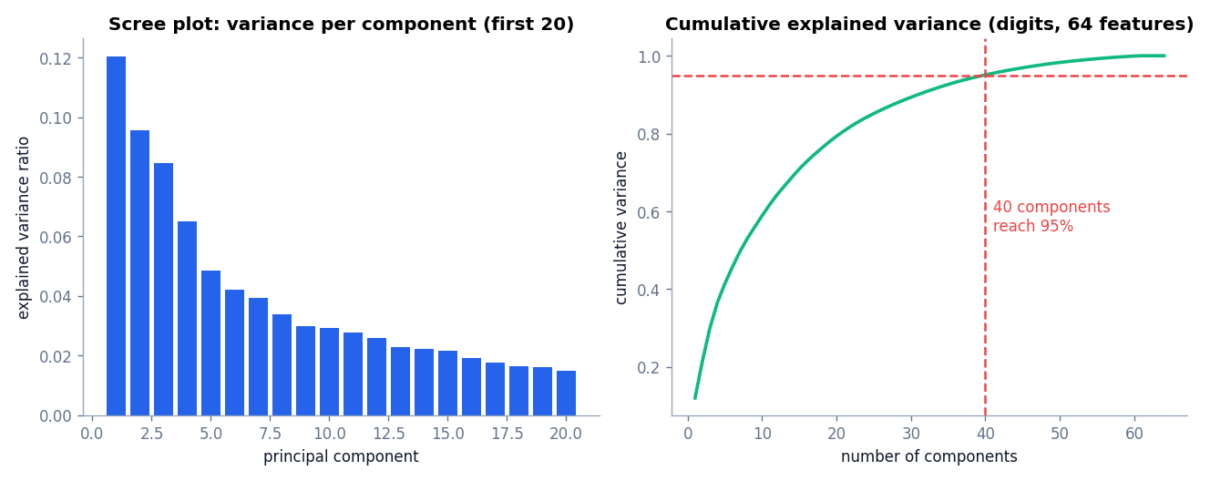
• The scree plot shows the variance of each component. Look for the point where the bars flatten out. Components after that point mostly carry fine detail or noise.
• The cumulative explained variance curve shows how much information you keep in total. Choose a target such as 90 or 95 percent, based on how much loss your task can tolerate.

There is no universal threshold. For visualization, you use two or three components regardless of the variance they carry. For preprocessing before a model, pick the smallest k that does not hurt downstream performance, and confirm it with validation.

Using PCA in a Machine Learning Pipeline

Take care with data leakage when PCA feeds a supervised model. PCA learns its mean, scaling, and components from data. If you fit it on the entire dataset before splitting into training and test sets, information from the test set leaks into the training process. Fit the scaler and PCA on the training set only, then apply the fitted transformations to the test set. In scikit-learn, put them inside a Pipeline so that cross-validation handles this correctly.

For clustering, PCA is a common step before K-means, because removing redundant dimensions makes distances more informative. The customer segmentation project uses PCA in the final article to draw cluster plots. The Gaussian mixture article also benefits, because fitting covariance matrices is easier in fewer dimensions.

PCA in practice: a short checklist

1. Inspect the data for missing values, because PCA cannot handle them.
2. Standardize numeric features unless they share the same units.
3. Fit PCA on training data only when a model evaluation follows.
4. Choose the number of components from the explained variance, not by habit.
5. Check the reconstruction error and the loadings before drawing conclusions.

Applications of PCA

• Visualization: projecting high-dimensional data into two or three dimensions to look for structure.
• Noise reduction: dropping low-variance components removes part of the noise.
• Compression: storing k scores per example instead of d original values.
• Preprocessing: decorrelating features and reducing dimensionality before clustering or modeling.
• Exploration: checking which original features contribute most to the main directions of variation.

Limitations of PCA

• It is linear. PCA only finds straight-line directions. Curved structures, such as a spiral, need nonlinear methods such as kernel PCA or autoencoders.
• Variance is not importance. A direction with high variance may be irrelevant to your task, and a low-variance direction may be the one that separates classes.
• Components are hard to interpret. Each component mixes all original features. You can inspect the components_ loadings, but the result is rarely a clean concept.
• Sensitive to scale and outliers. Unscaled features and extreme points can steer the components.
• Information is lost. Keeping fewer components always discards some variation.
• Plots can mislead. A two-dimensional PCA plot of data whose first two components carry only 22 percent of the variance can hide structure or suggest overlap that does not exist in the full space.

Common Mistakes

• Applying PCA without standardizing features that have different units.
• Fitting PCA on the full dataset before a train and test split.
• Interpreting a component as a single real-world factor without checking its loadings.
• Choosing the number of components without looking at the explained variance.
• Using PCA on categorical codes as if they were numeric measurements.

Frequently Asked Questions

Is PCA supervised or unsupervised?

Unsupervised. It uses only the features and never sees labels.

Does PCA select features?

No. Feature selection keeps a subset of the original columns. PCA creates new columns that are combinations of all the originals.

How many principal components should I keep?

Use the scree plot and the cumulative variance curve. Many projects target 90 to 95 percent of the variance. For plotting, keep two or three.

Why do I need to standardize before PCA?

PCA maximizes variance. A feature measured in large units has a large variance and would dominate the first component for reasons unrelated to its importance.

What is the difference between PCA and an autoencoder?

PCA learns a linear projection and has an exact mathematical solution. An autoencoder learns a possibly nonlinear compression with a neural network and needs training.

Conclusion

PCA rotates your data to a new set of axes ordered by how much variation they capture, then lets you keep only the first few. The covariance matrix and its eigenvectors give the directions, the eigenvalues give the variance, and the explained variance ratio tells you how much information you keep. Used with standardization and a leakage-safe pipeline, it is a fast and reliable way to simplify data.

PCA treats every cluster as a cloud with a direction and spread. A natural question is whether we can model each cluster as exactly that kind of cloud and assign points by probability. That is the idea behind Gaussian Mixture Models Explained: Soft Clustering Made Simple.

References

• scikit-learn documentation: Principal component analysis
• scikit-learn documentation: The digits dataset
• Pearson, K. (1901). On lines and planes of closest fit to systems of points in space. Philosophical Magazine, 2(11), 559 to 572.