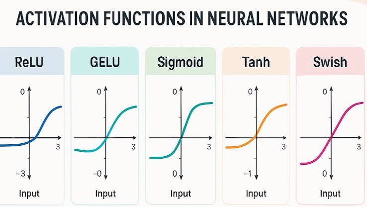
Activation Functions in Neural Networks: ReLU, Sigmoid, Softmax, and More
What Is an Activation Function? An activation function is a mathematical function that helps a neural network learn patterns from data. It takes a neuron’s calculated value as input and transforms that value into an output. Neural networks use activation functions to learn complex relationships between inputs and outputs. Without them, even a neural network with many layers would behave like a single linear model if every layer only performed a linear operation. For example, imagine you want to build a neural network that identifies cats and dogs in images. The network must learn patterns such as edges, shapes, ears, eyes, and fur. An activation function helps the network learn these complex patterns by introducing nonlinearity into its calculations. Different activation functions serve different purposes. Some work well in hidden layers, while others help the network produce probabilities for classification tasks. In this guide, you will learn how activation functions work, explore the most common types, compare their advantages and disadvantages, and understand how to choose the right one for a neural network. How Does an Activation Function Work? A neural network neuron receives input values, multiplies them by weights, adds a bias, and calculates a result. The neuron then passes this result through an activation function. A neuron typically calculates its output using two steps. Step 1: Calculate the weighted sum [ z = w_1x_1 + w_2x_2 + b ] Here: (x_1) and (x_2) represent input values. (w_1) and (w_2) represent weights. (b) represents the bias. (z) represents the weighted sum before activation. Step 2: Apply the activation function [ a = f(z) ] In this equation, (f) represents the activation function, and (a) represents the neuron’s output. Let’s use an example. Suppose a neuron calculates a weighted sum of 2. If the network uses the ReLU activation function, the neuron produces an output of 2. If the weighted sum equals -2, ReLU produces 0. This behavior allows the network to respond differently to different inputs. Why Do Neural Networks Need Activation Functions? Activation functions play an important role in neural network learning. They provide several benefits. 1. They introduce nonlinearity Real-world problems rarely follow simple linear relationships. Image recognition, speech processing, language understanding, and fraud detection all involve complex patterns. Activation functions allow neural networks to learn these nonlinear relationships. Without nonlinear activation functions, stacking multiple layers would not give a network the full learning power of a deep neural network. 2. They help neural networks learn complex patterns A neural network can combine the outputs of many neurons to identify increasingly complex features. Earlier layers may detect simple patterns, while deeper layers combine those patterns into more meaningful representations. Activation functions help the network build these representations during training. 3. They support different prediction tasks Different activation functions produce different output ranges. For example, sigmoid produces values between 0 and 1, which makes it useful for binary classification. Softmax converts a vector of scores into a probability distribution across multiple classes. The choice of activation function affects how the network learns and how it represents its predictions. Types of Activation Functions in Neural Networks Researchers and developers use several activation functions when building neural networks. The most common choices include ReLU, sigmoid, tanh, softmax, and newer functions such as GELU and Leaky ReLU. 1. ReLU Activation Function The ReLU activation function, which stands for Rectified Linear Unit, is one of the most widely used activation functions in deep learning. It returns the input value when the input is positive and returns zero when the input is negative. Its mathematical formula is: [ f(x) = \max(0,x) ] For example: If (x = 5), ReLU returns 5. If (x = 0), ReLU returns 0. If (x = -3), ReLU returns 0. ReLU has a simple calculation, which makes it computationally efficient. It also helps reduce the vanishing gradient problem for positive inputs compared with sigmoid and tanh. Advantages of ReLU It is simple and fast to calculate. It works well in many deep neural networks. It helps maintain stronger gradients for positive inputs. It often provides effective training performance in hidden layers. Disadvantages of ReLU ReLU can suffer from the dying ReLU problem. If a neuron repeatedly receives negative inputs, it may produce zero and stop learning through its usual gradient. This can make the neuron inactive during training. When should you use ReLU? Use ReLU as a starting choice for hidden layers in many feedforward neural networks and convolutional neural networks. Test alternatives when training performance or gradient behavior becomes a problem. 2. Sigmoid Activation Function The sigmoid activation function converts any real-valued input into a number between 0 and 1. Its formula is: [ f(x) = \frac{1}{1+e^{-x}} ] For example, sigmoid produces approximately 0.5 when the input equals zero. Large positive inputs produce values close to 1, while large negative inputs produce values close to 0. This output range makes sigmoid useful when a model needs to predict the probability of a binary outcome. Imagine a model that predicts whether an email is spam. It might produce a sigmoid output of 0.92, which indicates a predicted spam probability of 92%. Advantages of sigmoid It produces outputs between 0 and 1. It works well as an output activation for binary classification. It converts a single score into a probability-like value. Disadvantages of sigmoid Sigmoid can cause the vanishing gradient problem when its inputs become very positive or very negative. Its outputs can also make optimization slower in deep networks. When should you use sigmoid? Use sigmoid in the output layer of a binary classification model when you want one probability for a positive class. For training, developers commonly combine it with binary cross-entropy loss, often using a numerically stable implementation that accepts logits directly. 3. Tanh Activation Function The tanh activation function, also called the hyperbolic tangent function, maps input values to a range between -1 and 1. Its formula is: [ f(x) = \tanh(x) ] Tanh produces zero when the input equals zero. Positive inputs produce