Gaussian Mixture Models Explained: Soft Clustering Made Simple

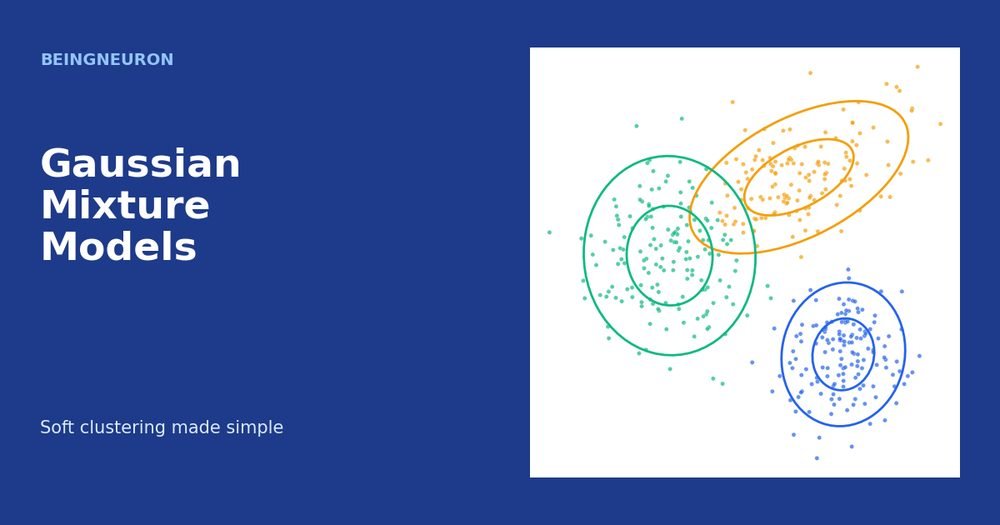
Gaussian Mixture Models (GMMs) are a probabilistic way to cluster data. Instead of drawing a hard border and saying “this point belongs to cluster 2”, a GMM says “this point is 70 percent likely to come from cluster 2 and 30 percent likely to come from cluster 3”. This is called soft clustering, and it is the main reason to choose a Gaussian mixture over K-means.

This article builds up the idea from a single bell curve to a mixture of several, explains the expectation-maximization (EM) algorithm that fits the model, shows how covariance types change cluster shapes, and uses AIC and BIC to choose the number of components. You will also implement EM from scratch for one-dimensional data and then use scikit-learn on two-dimensional data.

Hard Clustering vs Soft Clustering

K-means, hierarchical clustering, and DBSCAN return hard assignments: each point gets exactly one label. That is fine when groups are far apart. It hides information when groups overlap. A point sitting between two clusters gets the same label as a point deep inside one of them, and nothing in the output tells you the first assignment was a close call.

Soft clustering keeps that information. Each point receives a probability for every cluster, and the probabilities sum to one. You can still take the most likely cluster as a hard label, or you can use the uncertainty to flag ambiguous points for review.

Gaussian Distributions in Brief

A Gaussian distribution, also called a normal distribution, is the familiar bell curve. In one dimension it is described by a mean μ (the center) and a standard deviation σ (the spread). Its density is

N(x | μ, σ²) = (1 / √(2πσ²)) exp( −(x − μ)² / (2σ²) )

In several dimensions the mean becomes a vector μ and the spread becomes a covariance matrix Σ. The covariance matrix controls the size, the orientation, and the stretch of the cloud, so a two-dimensional Gaussian looks like an ellipse. Its density is

N(x | μ, Σ) = (2π)^−d/2 |Σ|^−1/2 exp( −½ (x − μ)^T Σ⁻¹ (x − μ) )

You do not need to evaluate this by hand. The point is that a Gaussian assigns the highest density near its mean and lower density as you move away, with the shape of the falloff set by Σ.

What Is a Gaussian Mixture Model?

A Gaussian mixture model assumes that the data was generated by K Gaussian distributions, called components, and that each data point came from exactly one of them. You never see which one. The model describes the overall density as a weighted sum:

p(x) = Σ_k=1..K π_k N(x | μ_k, Σ_k)

The mixing weights π_k are non-negative and add up to one. They give the fraction of the data that each component is responsible for.

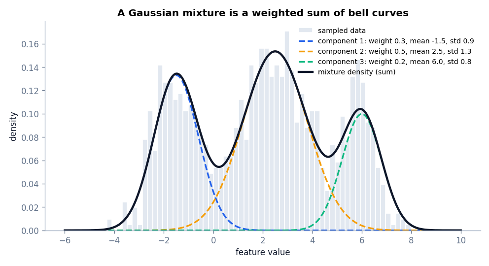
The figure shows three bell curves with weights 0.3, 0.5, and 0.2. Added together, they produce a density with several bumps, and that sum fits the histogram of the sampled data. Because the components overlap, a point in the overlapping region could plausibly have come from either one, which is exactly where soft clustering becomes useful.

Soft Cluster Membership

Once the model is fitted, Bayes’ rule gives the probability that point x came from component k. This probability is called the responsibility:

γ_k(x) = π_k N(x | μ_k, Σ_k) / Σ_j π_j N(x | μ_j, Σ_j)

The numerator is how strongly component k would produce the point, and the denominator normalizes the values so they sum to one.

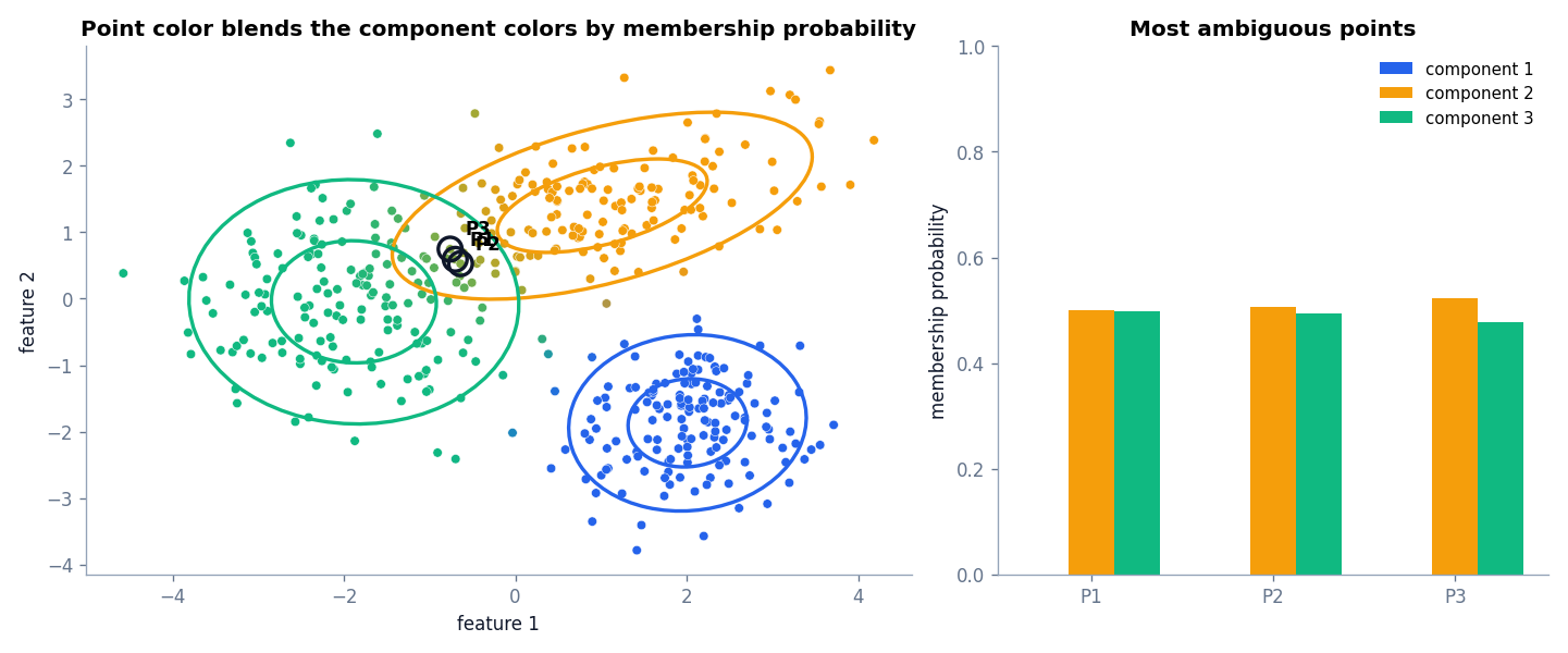
In the left panel, each point’s color blends the component colors according to its probabilities. Points deep inside an ellipse have a pure color. Points between ellipses have a mixed color. The bar chart shows the three most ambiguous points: each is about 50 percent likely to belong to component 2 and 50 percent to component 3. A hard-clustering algorithm would hide this.

The Expectation-Maximization Algorithm

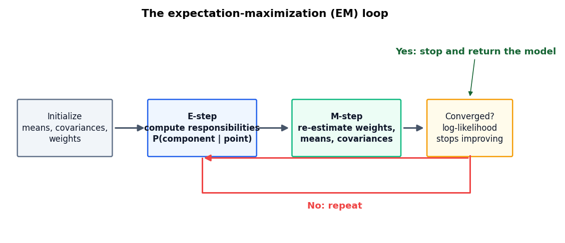
To fit a GMM you need to estimate the weights, means, and covariances. If you knew which component produced each point, this would be easy: just compute the mean and covariance of each group. If you knew the parameters, assigning points would be easy: just compute the responsibilities. You know neither, so the expectation-maximization (EM) algorithm alternates between the two.

1. Initialize the means, covariances, and weights, often with a short K-means run.
2. E-step (expectation): with the current parameters, compute the responsibility γ_ik of each component k for each point i.
3. M-step (maximization): re-estimate the parameters, treating responsibilities as soft counts.
4. Check convergence: compute the log-likelihood. If it has stopped improving, stop. Otherwise return to step 2.

The M-step updates are weighted versions of the usual formulas. With N_k = Σ_i γ_ik:

π_k = N_k / n,   μ_k = (1 / N_k) Σ_i γ_ik x_i,   Σ_k = (1 / N_k) Σ_i γ_ik (x_i − μ_k)(x_i − μ_k)^T

Compare the mean update with K-means. K-means averages the points that belong to a cluster. EM averages all points, each weighted by how much it belongs. K-means is the special case where responsibilities are forced to be 0 or 1.

EM from scratch for one-dimensional data

The script below generates 1,000 values from two bell curves, starts from rough guesses, and runs the E-step and M-step until the log-likelihood stops improving.

import numpy as np
from scipy.stats import norm

# 1D data from two bell curves: 60% from N(-1.5, 0.9^2) and 40% from N(3.0, 1.2^2).
rng = np.random.default_rng(0)
x = np.concatenate([rng.normal(-1.5, 0.9, 600), rng.normal(3.0, 1.2, 400)])

# Initial guesses (deliberately rough).
weights = np.array([0.5, 0.5])
means = np.array([-1.0, 1.0])
stds = np.array([1.0, 1.0])

previous = -np.inf
for step in range(1, 101):
    # E-step: responsibility of each component for each point (rows sum to 1).
    density = np.stack([w * norm.pdf(x, m, s) for w, m, s in zip(weights, means, stds)], axis=1)
    resp = density / density.sum(axis=1, keepdims=True)

    # M-step: re-estimate parameters using the responsibilities as soft counts.
    n_k = resp.sum(axis=0)
    weights = n_k / len(x)
    means = (resp * x[:, None]).sum(axis=0) / n_k
    stds = np.sqrt((resp * (x[:, None] - means) ** 2).sum(axis=0) / n_k)

    # Log-likelihood never decreases; stop when it stops improving.
    loglik = np.log(density.sum(axis=1)).sum()
    if step in (1, 2, 3, 5, 10) or abs(loglik - previous) < 1e-6:
        print(f"step {step:3d}  log-likelihood = {loglik:9.3f}")
    if abs(loglik - previous) < 1e-6:
        break
    previous = loglik

print("\nEstimated weights:", np.round(weights, 3), "(true 0.6, 0.4)")
print("Estimated means:  ", np.round(means, 3), "(true -1.5, 3.0)")
print("Estimated stds:   ", np.round(stds, 3), "(true 0.9, 1.2)")

step   1  log-likelihood = -2813.301
step   2  log-likelihood = -2069.087
step   3  log-likelihood = -2056.608
step   5  log-likelihood = -2043.367
step  10  log-likelihood = -2038.470
step  20  log-likelihood = -2038.444

Estimated weights: [0.604 0.396] (true 0.6, 0.4)
Estimated means:   [-1.508  2.923] (true -1.5, 3.0)
Estimated stds:    [0.909 1.108] (true 0.9, 1.2)

The log-likelihood rises from about −2,813 to about −2,038 and then stays flat, which shows convergence. EM never decreases the likelihood, but it can stop at a local optimum. The estimated weights (0.604, 0.396), means (−1.508, 2.923), and standard deviations (0.909, 1.108) are close to the true values used to create the data. They are not exact, because the sample is finite and the second component overlaps the first only slightly.

Covariance Types

The covariance matrix of each component decides its shape. scikit-learn offers four options through the covariance_type parameter.

Type	Shape of each component	Parameters
spherical	Circle, each with its own radius	Fewest
diag	Axis-aligned ellipse	Few
tied	Same ellipse shape and orientation for all components	Moderate
full	Any ellipse with its own size and rotation	Most

Full covariance is the most flexible and the default. It also needs the most data, because each component has a full covariance matrix with d(d + 1)/2 parameters. With few samples or many features, a simpler type is more stable.

Choosing the Number of Components With AIC and BIC

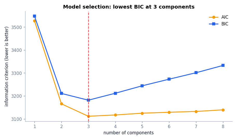
Like K-means, a GMM needs you to choose K. Because a GMM is a probability model, it has a principled tool for this. Adding components always raises the likelihood, so the likelihood alone would pick too many. The Akaike information criterion (AIC) and the Bayesian information criterion (BIC) subtract a penalty for model size:

AIC = 2p − 2 ln L,    BIC = p ln(n) − 2 ln L

Here L is the maximized likelihood, p is the number of free parameters, and n is the number of points. Lower is better for both. BIC penalizes complexity more strongly as n grows, so it tends to choose smaller models.

Gaussian Mixture Models in Python

The script below creates three overlapping groups, one of them stretched, and treats the group labels as unknown. It compares BIC and AIC for one to six components, fits a three-component model, prints the soft probabilities of the most uncertain points, compares covariance types, and measures agreement with K-means.

import numpy as np
from sklearn.datasets import make_blobs
from sklearn.mixture import GaussianMixture
from sklearn.cluster import KMeans
from sklearn.metrics import adjusted_rand_score

# Three overlapping groups; one is stretched so it is not a perfect circle.
X, y = make_blobs(n_samples=450, centers=[(-2.0, 0.0), (1.2, 1.2), (2.0, -1.8)],
                  cluster_std=[0.9, 0.8, 0.7], random_state=21)
X[y == 1] = X[y == 1] @ np.array([[1.4, 0.5], [0.0, 0.8]]) - np.array([0.7, 0.2])
# From here on we pretend y does not exist.

# Model selection: compare BIC and AIC for 1 to 6 components.
for k in range(1, 7):
    gm = GaussianMixture(n_components=k, covariance_type="full", n_init=5, random_state=21).fit(X)
    print(f"components={k}  BIC={gm.bic(X):8.1f}  AIC={gm.aic(X):8.1f}")

# Fit the chosen model.
gm = GaussianMixture(n_components=3, covariance_type="full", n_init=5, random_state=21).fit(X)
print("\nConverged:", gm.converged_, "after", gm.n_iter_, "EM iterations")
print("Mixing weights:", np.round(gm.weights_, 3))
print("Means:\n", np.round(gm.means_, 2))

# Hard labels versus soft probabilities.
hard = gm.predict(X)
soft = gm.predict_proba(X)
uncertain = np.argsort(soft.max(axis=1))[:3]
print("\nThree most uncertain points (membership probability per component):")
print(np.round(soft[uncertain], 2))
print("Points with max probability below 0.9:", int((soft.max(axis=1) < 0.9).sum()), "of", len(X))

# Covariance types change the shape each component may take.
print()
for cov in ["spherical", "diag", "tied", "full"]:
    m = GaussianMixture(n_components=3, covariance_type=cov, n_init=5, random_state=21).fit(X)
    print(f"{cov:9s} BIC = {m.bic(X):8.1f}")

# Compare the hard assignments with K-means (adjusted Rand index ignores label order).
km = KMeans(n_clusters=3, n_init=10, random_state=21).fit(X)
print("\nAgreement between K-means and GMM labels (ARI):", round(adjusted_rand_score(km.labels_, hard), 3))

components=1  BIC=  3547.6  AIC=  3527.1
components=2  BIC=  3210.9  AIC=  3165.7
components=3  BIC=  3181.6  AIC=  3111.7
components=4  BIC=  3210.2  AIC=  3115.7
components=5  BIC=  3243.2  AIC=  3124.1
components=6  BIC=  3271.6  AIC=  3127.8

Converged: True after 4 EM iterations
Mixing weights: [0.329 0.319 0.352]
Means:
 [[ 2.01 -1.87]
 [ 1.01  1.4 ]
 [-1.88 -0.05]]

Three most uncertain points (membership probability per component):
[[0.   0.5  0.5 ]
 [0.   0.51 0.49]
 [0.   0.52 0.48]]
Points with max probability below 0.9: 59 of 450

spherical BIC =   3208.2
diag      BIC =   3196.0
tied      BIC =   3206.9
full      BIC =   3181.6

Agreement between K-means and GMM labels (ARI): 0.916

How to read the results:

• BIC is lowest at three components (3181.6), and so is AIC (3111.7). Both agree with how the data was built. Two components underfit, and four or more add parameters without enough gain.
• EM converged after four iterations, and the mixing weights (0.329, 0.319, 0.352) are close to equal, as expected for 150 points per group.
• The three most uncertain points sit almost exactly on the boundary between two components, with probabilities near 0.5 and 0.5. 59 of the 450 points have a top probability below 0.9, so about 13 percent of the data is meaningfully ambiguous.
• Full covariance has the lowest BIC (3181.6), ahead of diag (3196.0), tied (3206.9), and spherical (3208.2). That is reasonable because one group was stretched into an ellipse.
• The adjusted Rand index of 0.916 shows that K-means and the GMM agree on most hard assignments. Their difference lies in the soft probabilities and the elliptical shapes, not in a different overall structure.

Key methods: fit runs EM, predict returns the most likely component, predict_proba returns the responsibilities, score_samples returns the log-density of each point, and sample generates new data from the fitted model. Because a GMM is a density model, it can also flag points with a very low density as anomalies, which connects to the anomaly detection article.

GMM vs K-Means

Aspect	K-means	Gaussian mixture
Assignment	Hard	Soft (probabilities)
Cluster shape	Round	Elliptical, depending on covariance type
Cluster size and spread	Assumed similar	Each component has its own
Choosing K	Elbow, silhouette	AIC, BIC, likelihood on held-out data
Speed	Faster	Slower, more parameters
Generative?	No	Yes, can sample new points

Hierarchical clustering is covered in its own article, and a GMM complements it when you want probabilities instead of a tree.

Applications

• Customer and market segmentation where segments overlap and probabilities are more honest than hard labels.
• Density estimation for modeling how a feature or set of features is distributed.
• Anomaly detection by flagging points with low likelihood.
• Speech and audio modeling, where GMMs have a long history.
• Image segmentation, grouping pixels by color distributions.

Limitations

• Gaussian assumption. If the true clusters are not roughly elliptical, such as crescents or rings, a GMM approximates them with several overlapping ellipses or fails. DBSCAN is a better fit there.
• Local optima. EM depends on initialization. Use n_init greater than 1 and a fixed random_state.
• Singular covariances. A component that collapses onto a few points can get a nearly singular covariance matrix and an enormous likelihood. scikit-learn guards against this with reg_covar.
• Number of components. AIC and BIC are guides, not proof. They can disagree, and they assume the Gaussian model is correct.
• High dimensions. Full covariance matrices have too many parameters for small samples. Reduce dimensions with PCA or use a restricted covariance type.
• Scale sensitivity. Standardize features when they use different units.

Common Mistakes

• Reading predicted probabilities as certain truth. They are model-based and depend on the Gaussian assumption.
• Choosing the number of components by training likelihood alone.
• Using full covariance on a small dataset with many features.
• Treating the component index as meaningful across runs. Component numbers can change between fits.
• Skipping the check against a simpler model such as K-means.

Frequently Asked Questions

What is the difference between K-means and a Gaussian mixture model?

K-means gives hard assignments to round clusters. A GMM gives membership probabilities and allows each cluster to have its own elliptical shape and size.

What does the EM algorithm do in a GMM?

It alternates between estimating how responsible each component is for each point (E-step) and updating the component parameters using those responsibilities (M-step) until the log-likelihood stops improving.

How do I pick the number of components?

Fit models with several values of K and compare their BIC or AIC. Choose the lowest value, then confirm that the components are interpretable.

Is a Gaussian mixture model supervised?

No. It is fitted without labels. Labels, if you have them, can only be used afterward to check the result.

Can a GMM detect outliers?

Yes. Points with very low density under the fitted model are candidates for outliers.

Conclusion

A Gaussian mixture model describes data as a blend of bell-shaped components and assigns each point a probability of belonging to each one. EM fits the model by alternating between soft assignments and parameter updates, covariance types control component shapes, and AIC or BIC guide the choice of K. Use it when clusters overlap, when they are elliptical, or when you need probabilities.

The probability view of data also helps with a different job: finding the points that do not fit any pattern at all. Continue with Anomaly Detection in Machine Learning: Finding Outliers in Unlabeled Data.

References

• scikit-learn documentation: Gaussian mixture models
• Dempster, A. P., Laird, N. M., and Rubin, D. B. (1977). Maximum likelihood from incomplete data via the EM algorithm. Journal of the Royal Statistical Society, Series B, 39(1), 1 to 38.
• Bishop, C. M. (2006). Pattern Recognition and Machine Learning, Chapter 9. Springer.