DBSCAN Clustering Explained: Core Points, Noise, and Outliers

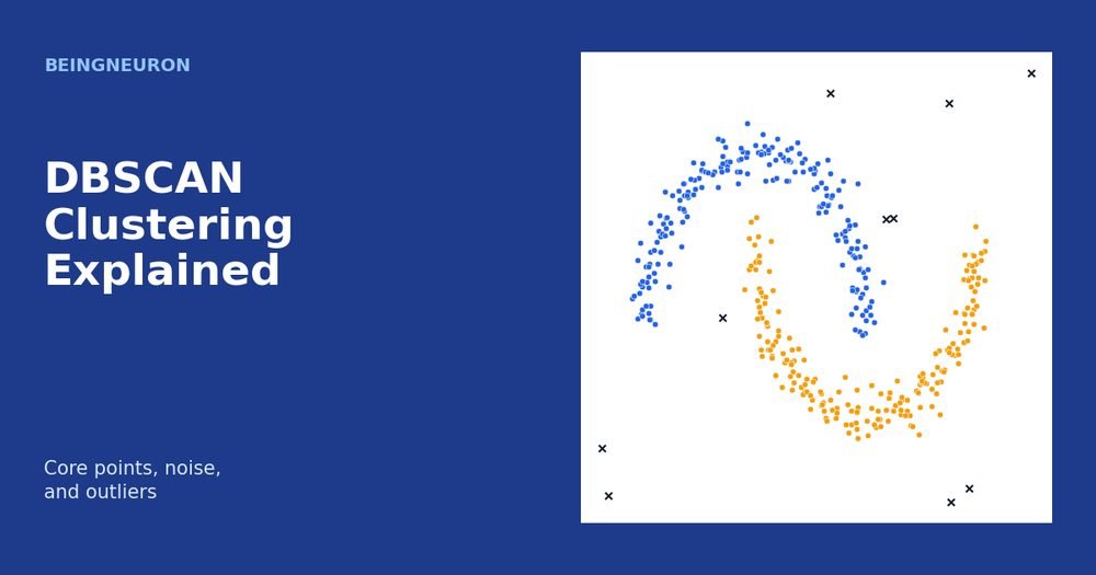
DBSCAN clustering groups points that sit in crowded regions of the data and labels points in sparse regions as noise. The name stands for Density-Based Spatial Clustering of Applications with Noise. Unlike K-means, it does not need the number of clusters in advance, it can find curved and irregular shapes, and it separates outliers instead of forcing them into a cluster.

This article explains how DBSCAN decides what counts as a cluster. You will learn the two parameters, the three types of points (core, border, and noise), the algorithm step by step, how to choose parameters with a k-distance plot, and how to run it in Python. It also covers where DBSCAN fails, which is just as important as where it works.

What Is Density-Based Clustering?

Centroid-based methods such as K-means describe a cluster by its center. Density-based methods describe a cluster as a region where points are packed closely together, separated from other regions by empty or sparse space.

Think of a map of city lights at night. Cities appear as bright dense patches, villages as smaller patches, and isolated farmhouses as lone dots. A density-based algorithm would call the patches clusters and the lone dots noise. It would not care whether a patch is round or shaped like a river valley.

The Two Parameters: Epsilon and Minimum Samples

DBSCAN has two parameters, and everything else follows from them.

• eps (ε): the radius of a neighborhood. Two points are neighbors if their distance is at most ε.
• min_samples: the number of points that must fall inside a point’s ε-neighborhood, including the point itself, for that area to count as dense.

The ε-neighborhood of a point p is the set of all points within distance ε of p:

N_ε(p) = { q : d(p, q) ≤ ε }

Core, Border, and Noise Points

Every point falls into exactly one of three types.

• Core point. Its ε-neighborhood contains at least min_samples points (counting itself). Core points lie in the interior of dense regions.
• Border point. It is not a core point, but it lies within ε of at least one core point. Border points sit on the edge of a cluster.
• Noise point. It is neither core nor border. No dense region reaches it.

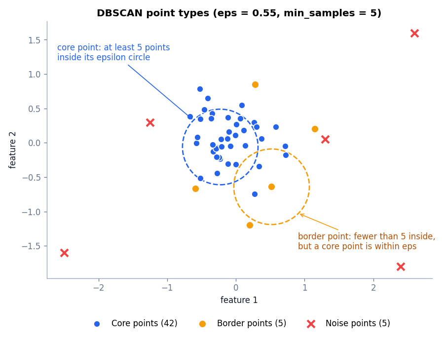
In the figure, the blue dashed circle is the ε-neighborhood of a core point and contains many points. The orange circle is centered on a border point. Fewer than five points fall inside it, so it is not a core point, yet it is close enough to a core point to join that cluster. The red crosses have no dense neighborhood anywhere near them, so DBSCAN marks them as noise. In this example the algorithm finds 42 core points, 5 border points, and 5 noise points.

How the DBSCAN Algorithm Works

Two ideas connect points into clusters.

• A point q is directly density-reachable from a point p if p is a core point and q is in the ε-neighborhood of p.
• Two points are density-connected if there is a chain of directly reachable core points that links them.

A cluster is a maximal set of density-connected points. The algorithm itself is short.

1. Pick any point that has not been visited.
2. Find its ε-neighborhood. If it has fewer than min_samples points, tentatively mark the point as noise and move on.
3. Otherwise, start a new cluster with this core point.
4. Add every neighbor to the cluster. For each neighbor that is also a core point, add its neighbors too, and keep expanding until no more points can be added.
5. Pick the next unvisited point and repeat until every point has been visited.

A point first marked as noise can later be claimed as a border point if a growing cluster reaches it. This is how border points are discovered. Because clusters grow by chaining, a cluster can follow a curve or ring of any shape.

A worked example in one dimension

Take six values on a number line: 1.0, 1.4, 1.9, 2.5, 3.2, and 8.0, with ε = 0.8 and min_samples = 3.

• 1.4 has neighbors 1.0 and 1.9 within 0.8, so with itself it has 3 points. It is a core point.
• 1.9 has neighbors 1.4 and 2.5, so it is a core point. 2.5 has neighbors 1.9 and 3.2, so it is also a core point.
• 1.0 has only 1.4 nearby, so it is not a core point. It is within 0.8 of the core point 1.4, so it is a border point. The same logic makes 3.2 a border point, because it is within 0.8 of the core point 2.5.
• 8.0 has no neighbors within 0.8, so it is noise.

The result is one cluster of five points (three core, two border) and one noise point. The cluster grew by chaining from one core point to the next, which is the mechanism that lets DBSCAN follow curves.

Why DBSCAN Handles Irregular Shapes

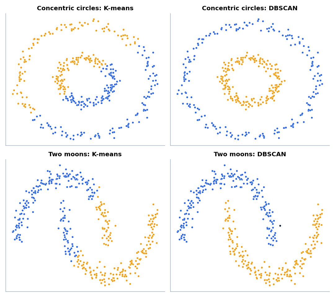
K-means assigns each point to the nearest centroid, so its cluster boundaries are straight lines between centroids. A ring around another ring cannot be separated that way. DBSCAN never uses centroids. It simply connects nearby dense points, so a ring or a crescent forms a single connected chain. In the figure, DBSCAN recovers both concentric circles and both crescents, while K-means splits each dataset down the middle.

How to Choose Epsilon and Minimum Samples

DBSCAN is sensitive to its parameters, so choose them deliberately.

Choosing min_samples

A common rule of thumb is min_samples ≥ d + 1 for d features, and often 2 * d for larger datasets. Larger values make the algorithm stricter, so more points become noise and clusters become more robust to outliers. For two-dimensional data, values between 4 and 10 are typical. If your data is noisy or very large, increase the value.

Choosing eps with a k-distance plot

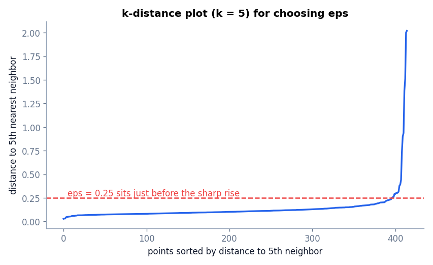
Set k equal to min_samples. For every point, compute the distance to its k-th nearest neighbor. Sort those distances from smallest to largest and plot them. Points inside clusters have small k-distances, while noise points have large ones, so the curve rises slowly and then sharply. A good ε sits near the bend of that curve.

DBSCAN in Python With scikit-learn

The script below builds two crescent-shaped clusters, adds 15 random points as noise, and standardizes the data. It then draws the k-distance statistics, tests several ε values, and fits the chosen model. You need numpy, matplotlib, and scikit-learn.

import numpy as np
import matplotlib.pyplot as plt
from sklearn.cluster import DBSCAN
from sklearn.datasets import make_moons
from sklearn.neighbors import NearestNeighbors
from sklearn.preprocessing import StandardScaler

# Two crescents plus 15 random points scattered across the plot as noise.
rng = np.random.default_rng(0)
moons, _ = make_moons(n_samples=400, noise=0.07, random_state=0)
scatter = rng.uniform([-1.5, -1.0], [2.5, 1.5], size=(15, 2))
X = StandardScaler().fit_transform(np.vstack([moons, scatter]))
print("Total points:", len(X))

# Step 1: k-distance plot to pick eps. Use k = min_samples.
min_samples = 5
distances, _ = NearestNeighbors(n_neighbors=min_samples).fit(X).kneighbors(X)
k_dist = np.sort(distances[:, -1])
print("k-distance percentiles (50, 90, 95, 99):", np.round(np.percentile(k_dist, [50, 90, 95, 99]), 3))

# Step 2: see how sensitive the result is to eps.
for eps in [0.1, 0.15, 0.2, 0.25, 0.3, 0.5]:
    lab = DBSCAN(eps=eps, min_samples=min_samples).fit(X).labels_
    print(f"eps={eps:.2f}  clusters={len(set(lab)) - (1 if -1 in lab else 0):2d}  noise={int((lab == -1).sum()):3d}")

# Step 3: fit the chosen model.
db = DBSCAN(eps=0.25, min_samples=min_samples).fit(X)
labels = db.labels_
n_clusters = len(set(labels)) - (1 if -1 in labels else 0)
print("Clusters found:", n_clusters)
print("Noise points:", int((labels == -1).sum()))
print("Core points:", len(db.core_sample_indices_))
print("Cluster sizes:", [int((labels == c).sum()) for c in sorted(set(labels)) if c != -1])

# Step 4: plot. Noise points get label -1.
for lab in sorted(set(labels)):
    mask = labels == lab
    if lab == -1:
        plt.scatter(X[mask, 0], X[mask, 1], c="black", marker="x", s=30, label="noise")
    else:
        plt.scatter(X[mask, 0], X[mask, 1], s=15, label=f"cluster {lab}")
plt.legend()
plt.title("DBSCAN result (black = noise)")
plt.show()

Total points: 415
k-distance percentiles (50, 90, 95, 99): [0.103 0.18  0.231 0.931]
eps=0.10  clusters=28  noise=119
eps=0.15  clusters= 5  noise= 32
eps=0.20  clusters= 3  noise= 12
eps=0.25  clusters= 2  noise= 10
eps=0.30  clusters= 2  noise= 10
eps=0.50  clusters= 1  noise=  7
Clusters found: 2
Noise points: 10
Core points: 396
Cluster sizes: [202, 203]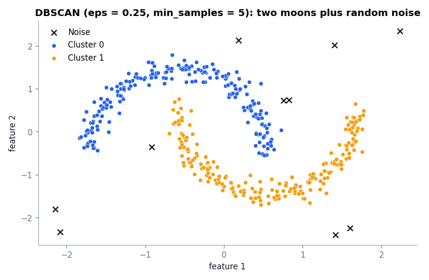

How to read the output:

• The k-distance percentiles show that most points have a fifth-neighbor distance below about 0.23, while the top percentile jumps to 0.93. That jump comes from the scattered noise points, and it suggests an ε around 0.2 to 0.3.
• The ε table shows how sensitive DBSCAN is. At ε = 0.10 the crescents break into 28 fragments and 119 points become noise. At ε = 0.50 everything merges into one cluster. Values of 0.25 and 0.30 recover the two crescents.
• The final model with ε = 0.25 finds two clusters of 202 and 203 points and labels 10 points as noise. Of the 15 random points, 10 fell far enough from the crescents to be noise, and the other five landed inside or next to a crescent and were absorbed into it. DBSCAN reports what the density says, not what we planted.

Important scikit-learn details

• labels_ contains one integer per point. The value −1 means noise.
• core_sample_indices_ holds the indices of core points. Border points are the clustered points that are not core.
• DBSCAN has no predict method for new data, because clusters are defined by the training points. Use fit_predict on a combined dataset, or train a classifier on the cluster labels if you need to label new points.
• Scale your features first. ε is a distance, so it only makes sense when all features share a comparable scale.

Advantages of DBSCAN

• No need to specify the number of clusters.
• Finds clusters of arbitrary shape.
• Identifies noise explicitly, which makes it useful as an outlier detector.
• Only two parameters, both with a clear geometric meaning.
• Efficient on moderately large datasets when a spatial index is used, with an average cost close to O(n log n).

Limitations of DBSCAN

• One density for all clusters. A single ε cannot fit a dense cluster and a sparse cluster at the same time. If ε suits the sparse one, the dense one may absorb its neighbors. If it suits the dense one, the sparse one dissolves into noise.
• Sensitivity to parameters. The ε table above shows how a small change can turn a clean result into fragments or a single blob.
• High dimensions. Distances become less informative as the number of features grows, so density is hard to define. Reduce dimensions first, for example with PCA.
• Border point ambiguity. A border point that lies within ε of two different clusters is assigned to whichever cluster reaches it first, so results can depend on data order for such points.
• No soft assignments. Every point is either in one cluster or labeled noise. For probabilities, see Gaussian Mixture Models.

If varying density is your problem, look at HDBSCAN (available in scikit-learn as sklearn.cluster.HDBSCAN) or OPTICS, which extend the density-based idea to clusters with different densities.

DBSCAN vs K-Means vs Hierarchical Clustering

Question	K-means	Hierarchical	DBSCAN
Number of clusters needed?	Yes	No (cut the tree)	No
Cluster shapes	Round	Depends on linkage	Arbitrary
Detects noise?	No	No	Yes
Varying densities?	Not applicable	Moderate	Weak
Main parameters	K	Linkage, cut height	eps, min_samples

Choose K-means for compact groups and large datasets. Choose hierarchical clustering when you want a tree. Choose DBSCAN when shapes are irregular, when you expect noise, or when you cannot guess the number of clusters.

Where DBSCAN Is Used

• Geospatial analysis: finding hot spots in location data, such as areas with many reported incidents.
• Anomaly detection: treating noise points as candidate anomalies. The anomaly detection article compares this idea with Isolation Forest and Local Outlier Factor.
• Image and sensor data: grouping dense regions of points, such as detections from a scanner.
• Data cleaning: flagging records that do not belong to any dense pattern.

A Practical DBSCAN Workflow

1. Standardize the features and, if there are many, reduce them with PCA.
2. Set min_samples from the rule of thumb for your number of features.
3. Draw the k-distance plot and pick an ε near the bend.
4. Fit the model and count clusters and noise points. Try a few nearby ε values, as the table above does, and prefer a value in a stable range.
5. Look at the noise points. If they are a meaningful share of the data, check whether ε is too small or whether the noise is real.

Common Mistakes

• Skipping feature scaling, so ε means different things in different directions.
• Choosing ε by trial without looking at a k-distance plot.
• Treating every noise point as a real anomaly. Noise only means “not in a dense region for these parameters”.
• Using one ε on data with clusters of very different density.
• Trying to call predict on new data.

Frequently Asked Questions

What does DBSCAN stand for?

Density-Based Spatial Clustering of Applications with Noise. It was introduced by Ester, Kriegel, Sander, and Xu in 1996.

What is the difference between a core point and a border point?

A core point has at least min_samples points inside its ε-neighborhood. A border point has fewer, but lies within ε of a core point, so it belongs to that point’s cluster.

How do I find the best eps value?

Plot the sorted distance to the k-th nearest neighbor with k equal to min_samples and choose ε near the sharp bend. Confirm by inspecting the clusters and the number of noise points.

Why does DBSCAN label everything as noise?

The most likely cause is that ε is too small, or min_samples is too large, for the scale of your data. Check that the data is scaled and increase ε.

Is DBSCAN better than K-means?

Neither is better in general. DBSCAN wins on irregular shapes and noisy data. K-means wins on speed, simplicity, and compact clusters.

Conclusion

DBSCAN defines clusters as dense regions connected through core points, marks isolated points as noise, and handles shapes that centroid methods cannot. Its two parameters need care, and its single density threshold is its main weakness. When the structure of your data is a puzzle of curves and noise, DBSCAN is often the first algorithm to try.

So far this series has grouped examples. The next article turns to the other side of the table and reduces the number of features with Principal Component Analysis (PCA) Explained with Python.

References

• scikit-learn documentation: DBSCAN
• Ester, M., Kriegel, H.-P., Sander, J., and Xu, X. (1996). A density-based algorithm for discovering clusters in large spatial databases with noise. Proceedings of KDD-96.