How Unsupervised Learning Works: Clustering, Patterns, and Data Structure

If you have read What Is Unsupervised Learning?, you know that these algorithms work without labels. The natural follow-up question is how unsupervised learning works and how it finds anything at all. Nobody tells the model what a group looks like, yet it returns clusters, patterns, and compressed views of the data.

This article explains how unsupervised learning works under the surface. The key ideas are features, similarity, distance, and an objective function that scores how well a model describes the data. Once these four ideas are clear, every algorithm in the rest of the series becomes easier to follow.

The Core Idea: Structure Comes From Similarity

Unsupervised algorithms rely on one assumption. If the data contains structure, similar examples will lie close together in some measurable sense, and different examples will lie farther apart. The algorithm turns that assumption into mathematics.

Every method answers three questions in some form:

1. How is each example represented as numbers?
2. How is “similar” measured?
3. What counts as a good description of the data?

The rest of this article takes these questions one at a time.

Features and Datasets

A dataset for unsupervised learning is a table. Each row is one example, also called a sample or observation. Each column is one feature, also called a variable or attribute. In notation, the table is a matrix X with n rows and d columns, and every row is a vector in d-dimensional space.

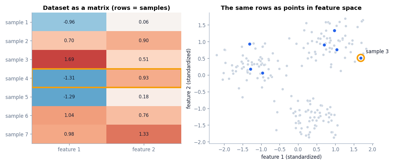
This view is what makes geometry possible. With two features you can plot points on a page. With 20 features you cannot draw the picture, but the mathematics is identical: each example is still a point, and distances between points still make sense.

What makes a good feature

The algorithm only sees the features you provide. If you want to group customers by behavior, features such as purchase frequency and average spend help. A customer ID does not, because it carries no behavioral meaning even though it is a number. Choosing features is the most influential decision in an unsupervised project.

Converting non-numeric data

Algorithms need numbers. Categories can be one-hot encoded, text can be converted to numeric embeddings, and images can be flattened into pixel values or encoded by a neural network. The quality of this conversion limits the quality of everything that follows.

Why Feature Scaling Changes the Result

Distance calculations add up differences across all features. If one feature has a much larger numeric range than the others, it dominates the sum. This is a frequent cause of clusters that look “wrong”.

The script below shows the effect. It compares three people described by age (in years) and income (in dollars), and then compares the three standard distance formulas on two simple points.

import numpy as np
from sklearn.preprocessing import StandardScaler
from scipy.spatial.distance import euclidean, cityblock, cosine

a = np.array([1.0, 1.0])
b = np.array([5.0, 4.0])
print("Euclidean:", round(euclidean(a, b), 3))
print("Manhattan:", round(cityblock(a, b), 3))
print("Cosine distance:", round(cosine(a, b), 3))

# Why scaling matters: income is in dollars, age is in years.
people = np.array([
    [25, 50000],   # person A
    [60, 51000],   # person B
    [26, 62000],   # person C
], dtype=float)

def dist(p, q):
    return np.linalg.norm(p - q)

print("\nRaw distances (age in years, income in dollars)")
print("A-B:", round(dist(people[0], people[1]), 1), "  A-C:", round(dist(people[0], people[2]), 1))

scaled = StandardScaler().fit_transform(people)
print("\nStandardized distances")
print("A-B:", round(dist(scaled[0], scaled[1]), 2), "  A-C:", round(dist(scaled[0], scaled[2]), 2))

Euclidean: 5.0
Manhattan: 7.0
Cosine distance: 0.006

Raw distances (age in years, income in dollars)
A-B: 1000.6   A-C: 12000.0

Standardized distances
A-B: 2.16   A-C: 2.21

In the raw data, person A and person B are 35 years apart in age but only $1,000 apart in income, so their distance is about 1,000. Person A and person C differ by one year but $12,000 in income, so their distance is 12,000. Income decides everything, and the 35-year age gap is invisible.

After standardization, each feature is rescaled to have mean 0 and standard deviation 1, using

z = (x − μ) / σ

where μ is the feature mean and σ is its standard deviation. The distances become 2.16 and 2.21, and both features now contribute on a comparable scale. Unless all your features already share the same units, scale before you use any distance-based method.

Measuring Similarity With Distance Metrics

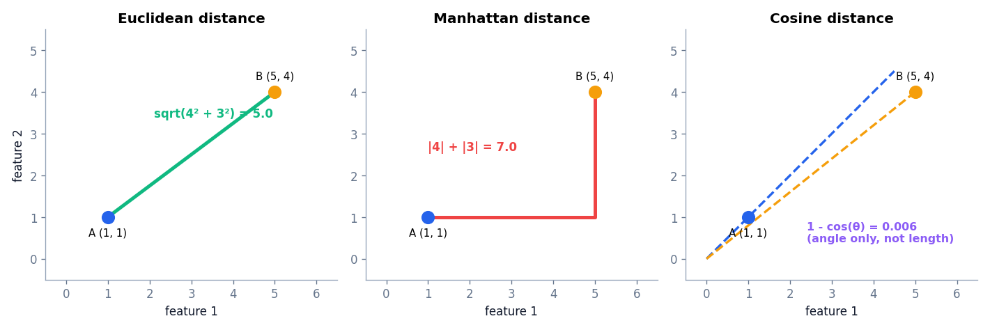
A distance metric turns two feature vectors into a single number. Small means similar and large means different. Three metrics cover most beginner projects.

Euclidean distance

This is the straight-line distance you would measure with a ruler.

d(x, y) = √( Σ_i (x_i − y_i)² )

For A = (1, 1) and B = (5, 4), the result is √(4² + 3²) = 5. K-means and Ward linkage are built around squared Euclidean distance.

Manhattan distance

Manhattan distance adds up the absolute differences along each axis, like walking along city blocks.

d(x, y) = Σ_i |x_i − y_i|

For the same two points the result is 4 + 3 = 7. It is less sensitive to a single large difference than Euclidean distance, which can help when a few features contain extreme values.

Cosine distance

Cosine distance ignores length and compares direction.

d(x, y) = 1 − (x · y) / (‖x‖ ‖y‖)

The two points above point in nearly the same direction, so their cosine distance is only 0.006 even though their Euclidean distance is 5. Cosine distance is popular for text and embeddings, where the length of a vector (for example, a longer document) is less important than which terms or concepts it contains.

Choosing a metric

• Use Euclidean distance as the default for scaled numeric features.
• Try Manhattan distance when outliers or many sparse features are a concern.
• Use cosine distance for text vectors and learned embeddings.

The metric is a modeling decision, not a detail. Changing it changes what the algorithm considers “similar”.

A warning about many dimensions

As the number of features grows, distances between points tend to become more alike. Nearest and farthest neighbors look almost equally far away, which weakens distance-based methods. This effect is part of the “curse of dimensionality”. It is one reason dimensionality reduction, covered in the PCA article, is often applied before clustering.

A Worked Example With Five Points

Consider five points in two dimensions: P1 = (1, 2), P2 = (2, 1), P3 = (8, 9), P4 = (9, 8), and P5 = (5, 5). The Euclidean distance between P1 and P2 is √(1² + 1²) = 1.41, and the same is true for P3 and P4. Those two pairs are obviously close, so any reasonable algorithm will group P1 with P2 and P3 with P4.

Now look at P5. Its distance to each of the other four points is exactly 5.0. It sits in the middle and is not closer to either group. A hard-clustering algorithm must still put it somewhere, which is one reason soft methods such as Gaussian mixtures exist, and why density-based methods such as DBSCAN can label a point like P5 as noise. This tiny example shows the whole idea of the section: structure is visible in the pattern of distances, and difficult points are the ones whose distances do not favor any group.

Other similarity measures

Not every feature is a measurement. For binary features, such as whether a customer bought each of 50 products, the Hamming distance counts the number of positions where two vectors differ, and the Jaccard distance compares the overlap of the sets of items that are present. For text, cosine distance on word or embedding vectors is common. Choose the measure that matches the data type, and check that the library function you use supports it.

How Clustering Discovers Hidden Structure

With features and a distance metric in place, clustering is easy to describe. The algorithm looks for a partition of the points in which distances inside each group are small compared with distances between groups.

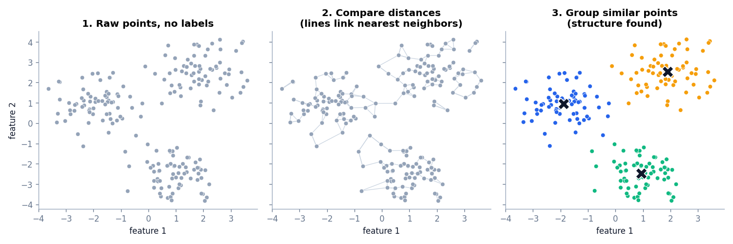
The figure walks through the idea. Panel one shows data with no labels. Panel two draws lines between each point and its nearest neighbors, which highlights that some regions are dense and others are empty. Panel three shows one possible result: three groups, each with a center.

The objective function

An algorithm needs a number that says how good a description is. That number is the objective function. The algorithm adjusts its parameters to improve the objective. Different methods optimize different objectives:

• K-means minimizes the total squared distance between each point and its cluster center.
• Hierarchical clustering repeatedly merges the pair of clusters that is closest under a chosen linkage rule.
• DBSCAN connects points that sit in dense neighborhoods and labels isolated points as noise.
• Gaussian mixtures maximize the likelihood of the data under a mixture of bell-shaped distributions.
• PCA finds new axes that keep as much variance as possible.

The algorithm never sees a right answer. It only sees whether the objective improved.

The Main Families of Methods

Centroid-based clustering

These methods describe each cluster by a center point. K-means is the best-known example. It is fast and simple but expects roughly round clusters of similar size.

Hierarchical clustering

These methods build a tree of nested clusters, so you can choose how coarse or fine the grouping should be. See Hierarchical Clustering Explained.

Density-based clustering

Here a cluster is a dense region separated from other dense regions by sparse space. DBSCAN can find curved shapes and mark outliers as noise.

Model-based clustering

These methods assume the data came from a mixture of probability distributions and estimate those distributions. Gaussian Mixture Models give each point a probability of belonging to each cluster.

Pattern Discovery Beyond Clustering

Dimensionality reduction

Real datasets often have more features than they need. Many features are correlated, and the information they carry overlaps. Dimensionality reduction finds a smaller set of features that preserves the most important variation. PCA does this with linear combinations of the original features. Autoencoders do it with neural networks and can capture nonlinear relationships.

Anomaly detection

If you can describe what normal data looks like, you can measure how far a new point is from normal. Anomaly detection methods score each example by how unusual it is.

How Do You Know the Result Is Good?

Without labels, there is no accuracy score. You evaluate in layers.

1. Internal metrics. The silhouette score and similar measures check how compact and well separated the clusters are. They are useful for comparing options on the same data, not for proving that a result is correct.
2. Stability. Re-run the algorithm on resampled data or with different random seeds. If the groups change wildly, they are probably not real structure.
3. Domain review. Look at each cluster and ask whether it makes sense. Can you describe how its members differ from the others? Does the description lead to an action?
4. External validation, when available. If you later obtain trusted labels or outcomes, you can compare the clusters against them. These labels must be used only for checking, never for training.

Putting It Together: A Typical Workflow

Most unsupervised projects follow the same order. Clean the data and select features, scale them, choose a distance metric, pick an algorithm that matches the expected structure, fit it with a fixed random seed, evaluate with internal metrics and stability checks, and finally interpret the result with a person who knows the domain. Each later article in this series is one concrete instance of this workflow.

Common Mistakes

• Skipping scaling. One large-range feature silently controls the result.
• Including meaningless features. IDs, timestamps stored as raw numbers, and duplicated columns distort distances.
• Trusting a single run. Many algorithms depend on random initialization. Use fixed seeds for reproducibility and several restarts for reliability.
• Forcing structure. K-means will return K clusters even if the data is one uniform cloud. Always plot the data or check stability.
• Ignoring outliers. A few extreme points can pull centers away from the true groups.

Frequently Asked Questions

How does unsupervised learning find patterns without labels?

It converts each example to a feature vector, measures similarity with a distance metric, and optimizes an objective that rewards a good description of the data, such as compact clusters or a high-variance projection.

What is the role of distance in unsupervised learning?

Distance defines similarity. Most clustering algorithms group points that are close and separate points that are far apart, so the choice of metric directly shapes the clusters.

Do I always need to scale my data?

For distance-based and variance-based methods, yes, unless all features already share the same units and range. Tree-based methods such as Isolation Forest are less sensitive to scale.

What is the difference between clustering and dimensionality reduction?

Clustering groups examples (rows). Dimensionality reduction compresses features (columns). Projects often use both, for example reducing dimensions first and clustering afterward.

How many clusters should I choose?

There is no universal rule. Combine a diagnostic such as the elbow method or silhouette score with domain judgment. The K-means article covers both techniques.

Conclusion

Unsupervised learning works by turning examples into points, measuring how close they are, and optimizing an objective that rewards a good description of that geometry. Features and scaling decide what the algorithm can see. The distance metric decides what counts as similar. The objective decides what counts as a good answer. When these three choices match your goal, the algorithms reveal useful structure. When they do not, the algorithms still return an answer, which is why careful validation matters.

Next, put these ideas into practice with the most popular clustering method in K-Means Clustering Explained with Examples and Python.

References

• scikit-learn documentation: Clustering
• scikit-learn documentation: Preprocessing data
• SciPy documentation: Distance computations