Linear Regression Explained with Examples

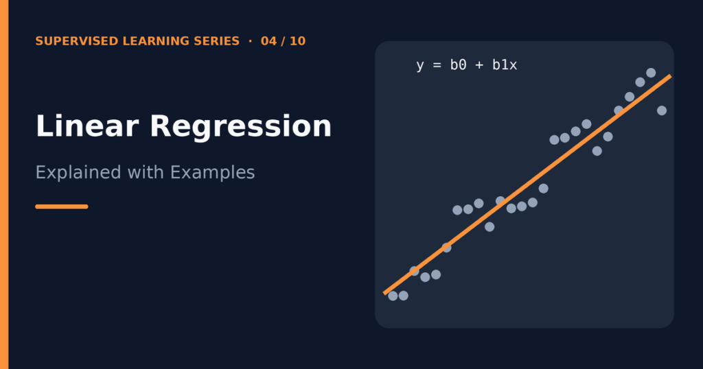
Linear regression is a supervised learning method that predicts a number by fitting a straight line (or, with several features, a flat plane) through your data. It finds the line that keeps the prediction errors as small as possible. Because the method is simple, fast, and easy to interpret, it is the standard first algorithm for anyone learning machine learning.

This guide explains linear regression with examples. You will see the equation, learn what coefficients and the intercept mean, work through a tiny least squares calculation by hand, understand gradient descent, and run a complete Python example. If you want background on the task type first, read Classification vs Regression in Machine Learning.

The core idea

Suppose you want to predict a house’s price from its size. You plot many past sales, with size on the horizontal axis and price on the vertical axis. The points rise from left to right but do not sit on a perfect line. Linear regression draws the one straight line that passes as close as possible to all the points. To predict a new house, you find its size on the line and read off the price.

With one feature, this is simple linear regression. With several features, such as size, bedrooms, and age, it is multiple linear regression. The idea stays the same: the prediction is a weighted sum of the features plus a starting value.

The linear regression equation

For one feature, the model is:

ŷ = β₀ + β₁x

Here is what each symbol means:

• ŷ (read “y-hat”) is the predicted value of the target.
• x is the feature, for example the house size.
• β₁ is the coefficient (also called the slope or weight). It tells you how much the prediction changes when x increases by one unit.
• β₀ is the intercept. It is the prediction when x equals zero.

For several features, you add one coefficient per feature:

ŷ = β₀ + β₁x₁ + β₂x₂ + … + βₚxₚ

Each coefficient describes the effect of its feature while the other features stay fixed. If β₁ equals 1.5 for house size in square meters, then each extra square meter adds 1.5 units to the predicted price, assuming the other features do not change. Be careful with the word “effect.” The model describes an association in the data. It does not prove that changing the feature would cause the target to change.

The intercept sometimes has no practical meaning. A house of zero square meters does not exist, so the intercept simply positions the line.

Loss function and the best-fit line

Infinitely many lines pass through a cloud of points. To choose the best one, we need a way to score each line. That score is the loss function, and linear regression usually uses the sum or mean of squared errors.

For each training example, the residual is the difference between the true value and the predicted value: residual = y − ŷ. Squaring the residuals makes every error positive, so errors above and below the line cannot cancel each other out. Squaring also punishes large errors more than small ones. The mean squared error is:

MSE = (1/n) × Σ (yᵢ − ŷᵢ)²

Here n is the number of examples, and Σ means “add up over all examples.” The best-fit line is the one with the smallest MSE. This approach is called ordinary least squares (OLS).

Least squares: a worked example

You can find the best line with a short calculation. Take three points: (1, 2), (2, 4), and (3, 5), where the first number is x and the second is y.

1. Compute the means: x̄ = 2 and ȳ = 11/3 ≈ 3.667.
2. Compute the slope with β₁ = Σ(x − x̄)(y − ȳ) / Σ(x − x̄)². The numerator is (−1)(−1.667) + (0)(0.333) + (1)(1.333) = 3. The denominator is 1 + 0 + 1 = 2. So β₁ = 1.5.
3. Compute the intercept with β₀ = ȳ − β₁x̄ = 3.667 − 1.5 × 2 ≈ 0.667.

The fitted line is ŷ = 0.667 + 1.5x. Its predictions for the three points are about 2.167, 3.667, and 5.167. The residuals are about −0.167, 0.333, and −0.167, and the sum of their squares is about 0.167. No other straight line gives a smaller sum for these three points.

For large datasets and many features, software solves the same problem with matrix algebra. Scikit-learn’s LinearRegression does exactly that, so you rarely calculate it yourself.

Gradient descent

The least squares formula gives the answer in one step for linear regression. However, many other models have no such formula, so machine learning often uses gradient descent, an iterative method. Linear regression is the classic way to learn it.

Picture the loss as a hilly landscape, where each position is a pair of values (β₀, β₁) and the height is the MSE. You start at a random position and take small steps downhill until you reach the bottom. At each step, you:

1. Calculate the gradient, which points in the direction where the loss grows fastest.
2. Move each parameter a small step in the opposite direction.

The update rule is β ← β − α × (gradient). The symbol α is the learning rate, which controls the step size. If α is too small, training is slow. If α is too large, the steps overshoot and the loss may grow instead of shrink. For linear regression with squared error, the loss surface is bowl-shaped, so gradient descent heads toward a single global minimum rather than getting stuck in local dips.

Gradient descent matters most for huge datasets, where a direct solution is slow, and for models with no direct solution. In scikit-learn, the SGDRegressor class uses a stochastic version. Features should be scaled before using it so that the steps behave well.

Assumptions of linear regression

Linear regression works best when the data roughly follow these conditions:

• Linearity. The relationship between the features and the target is approximately a straight line (or plane).
• Independent errors. One example’s error does not depend on another’s. Time series data often breaks this rule.
• Constant spread of errors. The size of the errors stays similar across the range of predictions. Statisticians call this homoscedasticity.
• Roughly normal errors. This matters mostly when you want confidence intervals and statistical tests. It matters less for pure prediction.
• No severe multicollinearity. Features that are almost copies of each other make the coefficients unstable and hard to interpret.

A residual plot, which plots residuals against predictions, is the easiest check. You want a shapeless cloud around zero. A curve or a funnel shape signals a problem.

Evaluation metrics

After training, you evaluate the model on a test set. Four regression metrics are standard:

• MAE (mean absolute error) is the average absolute error. It uses the same units as the target and is easy to explain.
• MSE (mean squared error) is the average squared error. It is the quantity the model minimizes.
• RMSE (root mean squared error) is the square root of MSE. It returns to the target’s units but weights big errors more than MAE does.
• R² (R-squared) is the share of the target’s variation that the model explains. A value near 1 means a strong fit. A value near 0 means the model does little better than predicting the average. R² can even be negative on test data when the model does worse than that.

The article on how to evaluate a supervised learning model compares these metrics in more depth.

Working Python example

This example creates a synthetic housing dataset so that you know the true relationship. The true rule is price = 20 + 1.5 × size, plus random noise. The price is in thousands, and the size is in square meters. We then check how close the model gets.

import numpy as np
from sklearn.linear_model import LinearRegression
from sklearn.model_selection import train_test_split
from sklearn.metrics import mean_absolute_error, mean_squared_error, r2_score

rng = np.random.default_rng(42)
size = rng.uniform(50, 250, 200)                 # house size in square meters
price = 20 + 1.5 * size + rng.normal(0, 25, 200) # price in thousands, with noise
X = size.reshape(-1, 1)                          # scikit-learn expects a 2D feature array
X_train, X_test, y_train, y_test = train_test_split(
    X, price, test_size=0.2, random_state=42)

model = LinearRegression().fit(X_train, y_train)
pred = model.predict(X_test)

print("Intercept:", round(float(model.intercept_), 2))
print("Coefficient:", round(float(model.coef_[0]), 3))
print("MAE:", round(mean_absolute_error(y_test, pred), 2))
print("RMSE:", round(float(np.sqrt(mean_squared_error(y_test, pred))), 2))
print("R2:", round(r2_score(y_test, pred), 3))
print("Prediction for 120 sq m:", round(float(model.predict([[120]])[0]), 1))

Required packages are numpy and scikit-learn. When I ran this code with Python 3.12 and scikit-learn 1.8.0, it printed:

Intercept: 5.94
Coefficient: 1.585
MAE: 20.01
RMSE: 25.38
R2: 0.911
Prediction for 120 sq m: 196.2

Here is how to read the result:

• The learned coefficient (1.585) is close to the true value (1.5), and the intercept (5.94) differs from the true value (20) by a noticeable margin. Random noise and a limited sample explain the gap. The intercept is harder to pin down here because the data never includes houses near zero square meters.
• The MAE of about 20 means the predictions miss by around 20 thousand on average. The RMSE of about 25 matches the noise level we added (a standard deviation of 25), which is what we should expect from a model that has learned the true pattern.
• An R² of 0.911 means the model explains about 91% of the price variation in the test set.

Notice that the code trains on X_train only and evaluates on X_test. See Training Data vs Testing Data for why that separation matters. Your numbers may differ slightly with other library versions.

Limitations

• It only captures straight-line relationships. You can add polynomial or interaction features, but you must choose them yourself.
• Outliers pull the line. Because errors are squared, a few extreme points can shift the fit a lot.
• It extrapolates poorly. The line keeps going forever, even where real data would stop following the pattern.
• Correlated features confuse coefficients. Predictions may stay fine while individual coefficients become unreliable.
• It cannot classify directly. For yes-or-no targets, use logistic regression instead.

Regularized versions, called ridge and lasso regression, add a penalty on large coefficients. They help when you have many features or correlated features.

Frequently asked questions

What is linear regression used for?

People use it to predict numeric values, such as prices, demand, or temperatures, and to measure how strongly each feature is associated with the target. It is also a common baseline that more complex models must beat.

What is the difference between simple and multiple linear regression?

Simple linear regression uses one feature. Multiple linear regression uses two or more features. The equation has one coefficient per feature, plus the intercept.

What does a high R-squared mean?

It means the model explains a large share of the variation in the target. It does not prove that the model is correct or that the features cause the target. Always check R² on test data and look at residuals.

Do I need to scale features for linear regression?

Ordinary least squares does not require scaling to find the right answer. Scaling helps when you use gradient descent or regularization, and it makes coefficients easier to compare.

Is least squares or gradient descent better?

For small and medium datasets, the direct least squares solution is fast and exact. Gradient descent shines with very large datasets or models that have no direct solution. Both aim at the same minimum for linear regression.

Conclusion

Linear regression fits a line by minimizing squared errors. The intercept and coefficients tell you how the prediction responds to each feature, and metrics such as MAE, RMSE, and R² tell you how well the line performs on unseen data. Understanding it well gives you the foundation for loss functions, optimization, and regularization, which appear again in almost every other algorithm.

Next, learn how a similar equation can predict categories in Logistic Regression Explained for Beginners.

This article is for educational and informational purposes only. Examples and code are provided to help readers understand linear regression and may require adaptation for specific projects.

Related guides

Compare linear regression with logistic regression, and see how regression differs from classification in Classification vs Regression in Machine Learning.

References and further reading

• Linear Models in the scikit-learn user guide for ordinary least squares, ridge, and lasso.
• Metrics and scoring in the scikit-learn user guide for MAE, MSE, and R².