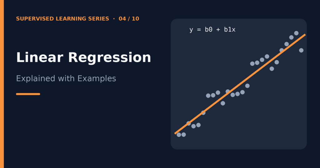
Linear Regression

Linear regression is a supervised learning method that predicts a number by fitting a straight line (or, with several features, a flat plane) through your data. It finds the line that keeps the prediction errors as small as possible. Because the method is simple, fast, and easy to interpret, it is the standard first algorithm for anyone learning machine learning. This guide explains linear regression with examples. You will see the equation, learn what coefficients and the intercept mean, work through a tiny least squares calculation by hand, understand gradient descent, and run a complete Python example. If you want background on the task type first, read Classification vs Regression in Machine Learning. Table of contents The core idea The linear regression equation Loss function and the best-fit line Least squares: a worked example Gradient descent Assumptions of linear regression Evaluation metrics Working Python example Limitations Frequently asked questions Conclusion The core idea Suppose you want to predict a house’s price from its size. You plot many past sales, with size on the horizontal axis and price on the vertical axis. The points rise from left to right but do not sit on a perfect line. Linear regression draws the one straight line that passes as close as possible to all the points. To predict a new house, you find its size on the line and read off the price. With one feature, this is simple linear regression. With several features, such as size, bedrooms, and age, it is multiple linear regression. The idea stays the same: the prediction is a weighted sum of the features plus a starting value. The linear regression equation For one feature, the model is: ŷ = β₀ + β₁x Here is what each symbol means: ŷ (read “y-hat”) is the predicted value of the target. x is the feature, for example the house size. β₁ is the coefficient (also called the slope or weight). It tells you how much the prediction changes when x increases by one unit. β₀ is the intercept. It is the prediction when x equals zero. For several features, you add one coefficient per feature: ŷ = β₀ + β₁x₁ + β₂x₂ + … + βₚxₚ Each coefficient describes the effect of its feature while the other features stay fixed. If β₁ equals 1.5 for house size in square meters, then each extra square meter adds 1.5 units to the predicted price, assuming the other features do not change. Be careful with the word “effect.” The model describes an association in the data. It does not prove that changing the feature would cause the target to change. The intercept sometimes has no practical meaning. A house of zero square meters does not exist, so the intercept simply positions the line. Loss function and the best-fit line Infinitely many lines pass through a cloud of points. To choose the best one, we need a way to score each line. That score is the loss function, and linear regression usually uses the sum or mean of squared errors. For each training example, the residual is the difference between the true value and the predicted value: residual = y − ŷ. Squaring the residuals makes every error positive, so errors above and below the line cannot cancel each other out. Squaring also punishes large errors more than small ones. The mean squared error is: MSE = (1/n) × Σ (yᵢ − ŷᵢ)² Here n is the number of examples, and Σ means “add up over all examples.” The best-fit line is the one with the smallest MSE. This approach is called ordinary least squares (OLS). Least squares: a worked example You can find the best line with a short calculation. Take three points: (1, 2), (2, 4), and (3, 5), where the first number is x and the second is y. Compute the means: x̄ = 2 and ȳ = 11/3 ≈ 3.667. Compute the slope with β₁ = Σ(x − x̄)(y − ȳ) / Σ(x − x̄)². The numerator is (−1)(−1.667) + (0)(0.333) + (1)(1.333) = 3. The denominator is 1 + 0 + 1 = 2. So β₁ = 1.5. Compute the intercept with β₀ = ȳ − β₁x̄ = 3.667 − 1.5 × 2 ≈ 0.667. The fitted line is ŷ = 0.667 + 1.5x. Its predictions for the three points are about 2.167, 3.667, and 5.167. The residuals are about −0.167, 0.333, and −0.167, and the sum of their squares is about 0.167. No other straight line gives a smaller sum for these three points. For large datasets and many features, software solves the same problem with matrix algebra. Scikit-learn’s LinearRegression does exactly that, so you rarely calculate it yourself. Gradient descent The least squares formula gives the answer in one step for linear regression. However, many other models have no such formula, so machine learning often uses gradient descent, an iterative method. Linear regression is the classic way to learn it. Picture the loss as a hilly landscape, where each position is a pair of values (β₀, β₁) and the height is the MSE. You start at a random position and take small steps downhill until you reach the bottom. At each step, you: Calculate the gradient, which points in the direction where the loss grows fastest. Move each parameter a small step in the opposite direction. The update rule is β ← β − α × (gradient). The symbol α is the learning rate, which controls the step size. If α is too small, training is slow. If α is too large, the steps overshoot and the loss may grow instead of shrink. For linear regression with squared error, the loss surface is bowl-shaped, so gradient descent heads toward a single global minimum rather than getting stuck in local dips. Gradient descent matters most for huge datasets, where a direct solution is slow, and for models with no direct solution. In scikit-learn, the SGDRegressor class uses a stochastic version. Features should be scaled before using it