decision trees

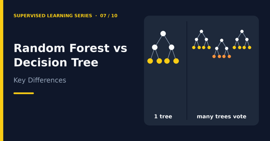
The main difference in random forest vs decision tree is simple: a decision tree is one model that asks a chain of questions, while a random forest is a team of many decision trees whose predictions are combined. A single tree is easy to read but unstable. A forest is usually more accurate and more stable, but harder to interpret and more expensive to run. This guide explains both models, shows how bootstrap sampling, feature randomness, and bagging create a forest, and compares them on accuracy, interpretability, cost, and feature importance. A Python comparison with real output follows. If you have not met single trees yet, start with Decision Trees in Machine Learning: How They Work. Table of contents Random forest vs decision tree at a glance A quick look at the decision tree Ensemble learning in plain English How a random forest works Key differences explained Feature importance Practical comparison in Python When to use each model Limitations of random forests Frequently asked questions Conclusion Random forest vs decision tree at a glance Aspect Decision tree Random forest What it is A single tree An ensemble of many trees Prediction The value in one leaf The combined result of all trees Overfitting High risk when the tree is deep Lower risk, because averaging reduces variance Accuracy Often lower Often higher Stability Small data changes can alter the tree More stable across data changes Interpretability High: you can read the whole tree Lower: hundreds of trees are hard to inspect Training and prediction cost Low Higher, roughly proportional to the number of trees Main settings Depth, leaf size, pruning Number of trees, features per split, plus tree settings A quick look at the decision tree A decision tree splits the data again and again with simple questions until it reaches leaves that hold predictions. It works for classification and regression, it needs no feature scaling, and you can display it as a flowchart. Its weakness is high variance. If you change a few training rows, the best first question may change, and the whole tree can look different. A deep tree also tends to memorize noise. You can read about this in Overfitting vs Underfitting in Machine Learning. Ensemble learning in plain English Ask one person to guess the number of candies in a jar, and the answer may be far off. Ask 200 people, average the guesses, and the result is usually much closer. Individual mistakes point in different directions, so they partly cancel out. This is the idea behind ensemble learning: combine several models so that the group performs better than a typical member. The trick only works if the members make different mistakes. A hundred identical trees would just repeat the same errors. A random forest therefore uses two sources of randomness to make the trees differ. How a random forest works Bootstrap sampling For each tree, the algorithm draws a random sample of the training rows with replacement. That means a row can appear several times in one sample, and other rows can be missing. If the original dataset has n rows, each bootstrap sample also has n rows, and on average about 63% of the distinct original rows appear in it. Every tree therefore trains on a slightly different dataset. Bagging Bagging is short for bootstrap aggregating. It means training each model on its own bootstrap sample and then aggregating the predictions. Bagging alone, applied to decision trees, already reduces variance. Feature randomness A random forest adds a second source of randomness. At every split inside every tree, the algorithm considers only a random subset of the features instead of all of them. This stops one strong feature from dominating every tree. As a result, the trees look less alike, and their errors are less correlated. In scikit-learn, the max_features parameter controls the subset size. For classifiers the default is the square root of the number of features. For regressors the default uses all features, so you may want to tune it. Prediction aggregation To predict, the forest sends the example through every tree and combines the results. For regression, it averages the predicted numbers. For classification, the classic description is majority voting. Scikit-learn’s implementation averages the class probabilities from the trees and picks the class with the highest average, which is a softer form of voting. Out-of-bag evaluation Each tree never sees the rows left out of its bootstrap sample. Those rows are called out-of-bag samples, and you can use them to estimate performance without a separate validation set. In scikit-learn, set oob_score=True. Still keep a real test set for the final check, as described in Training Data vs Testing Data. Key differences explained Accuracy and generalization A random forest usually generalizes better than a single tree. Averaging many different trees cancels much of the noise that a single deep tree memorizes. The improvement is not guaranteed, so compare both models on your own data with cross-validation. On very small or very clean datasets, a well-tuned single tree can come close. Interpretability A single tree wins here. You can print its rules and explain a prediction by naming one path. A forest of 200 trees has no single path to explain. You can still summarize it with feature importance scores and other tools, but you lose the simple flowchart. Computational cost A forest trains many trees, so it takes longer and uses more memory than a single tree. Prediction time also grows with the number of trees. The trees are independent, so scikit-learn can train them in parallel when you set n_jobs. For most beginner datasets the cost is small, but it can matter on large data or in systems that must answer in milliseconds. Tuning effort A forest often gives good results with default settings, which is a practical advantage. Important settings include n_estimators (the number of trees), max_features, max_depth, and min_samples_leaf. More trees rarely cause overfitting, but they stop helping after a point. Feature importance A forest can report how useful