Autoencoders Explained: How Neural Networks Learn Without Labels

Autoencoders are neural networks that learn to copy their input to their output through a narrow bottleneck. That sounds pointless until you notice the catch: because the bottleneck is small, the network cannot memorize every detail. It has to learn a compact summary of the data, and that summary, called the latent representation, is what makes autoencoders useful.

No labels are needed. The input is also the target, which is why autoencoders count as unsupervised (or, in current terminology, self-supervised) learning. This article explains the encoder and decoder, the latent space, the reconstruction loss, and the training process. You will then build a small autoencoder in PyTorch, view its reconstructions, and use it to detect anomalies. The article assumes you have seen PCA, because autoencoders can be understood as a nonlinear relative of it.

What Is an Autoencoder?

An autoencoder has two connected parts:

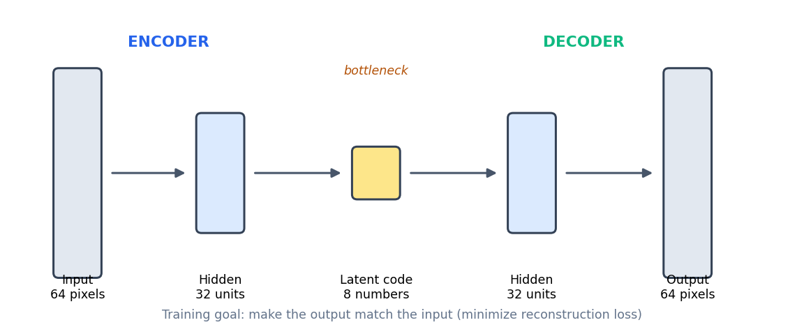
• The encoder compresses the input x into a short vector z, called the latent representation or code.
• The decoder reconstructs an approximation x̂ of the input from z.

In formulas, z = f(x) and x̂ = g(z), where f is the encoder network and g is the decoder network. The network is trained so that x̂ is as close to x as possible.

Why Compress and Rebuild?

If the latent code were as large as the input, the network could learn a trivial identity function and learn nothing useful. A bottleneck forces it to keep only the information that matters for rebuilding the input. For data with structure, such as images of digits, the structure is exactly what survives. The code ends up describing things like stroke direction and thickness instead of individual pixel values.

An autoencoder with a bottleneck smaller than the input is called undercomplete. There are also overcomplete autoencoders whose code is larger than the input. These need other constraints, such as noise added to the input (denoising autoencoders) or a sparsity penalty, to prevent them from copying the input without learning.

Reconstruction Loss

The training objective is the reconstruction loss, a measure of how different the output is from the input. For continuous data such as pixel intensities, the standard choice is mean squared error:

L = (1 / n) Σ_i=1..n ‖x_i − x̂_i‖²

Binary cross-entropy is another option when inputs lie between 0 and 1 and can be read as probabilities. The loss is computed per example, which also gives a natural per-example error score. That score is the key to anomaly detection later in this article.

How Training Works

1. Feed a batch of inputs through the encoder to get codes.
2. Feed the codes through the decoder to get reconstructions.
3. Compute the loss between reconstructions and the original inputs.
4. Use backpropagation to compute how each weight affects the loss.
5. Update the weights with an optimizer such as Adam.
6. Repeat for many batches and epochs.

The only thing that makes this unusual is step 3: the target is the input itself, so no labeled dataset is required.

A Beginner-Friendly PyTorch Implementation

The example uses scikit-learn’s digits dataset, which contains 1,797 grayscale images of handwritten digits, each 8 by 8 pixels. Pixel values range from 0 to 16, so the script divides by 16 to get values between 0 and 1. Install the dependencies with pip install torch scikit-learn numpy.

The experiment is designed to test both reconstruction and anomaly detection. The script holds out every image of the digit 9 and trains only on digits 0 to 8. The labels are used just to build this experiment. The autoencoder itself never receives a label.

import numpy as np
import torch
from torch import nn
from sklearn.datasets import load_digits
from sklearn.model_selection import train_test_split
from sklearn.metrics import roc_auc_score

torch.manual_seed(42)
np.random.seed(42)

# 1. Data: 8x8 digit images scaled to [0, 1].
digits = load_digits()
X = digits.data / 16.0
y = digits.target

# For a controlled anomaly demo we hold out every "9". Labels are used ONLY to build
# this experiment; the autoencoder itself never sees a label.
is_normal = y != 9
X_train, X_test, y_train, y_test = train_test_split(
    X[is_normal], y[is_normal], test_size=0.25, random_state=42, stratify=y[is_normal])
X_anom = X[~is_normal]
print("Train:", X_train.shape, " Test (normal):", X_test.shape, " Anomalies:", X_anom.shape)

# 2. Model: 64 -> 32 -> 8 (latent) -> 32 -> 64.
class Autoencoder(nn.Module):
    def __init__(self, n_inputs=64, n_hidden=32, n_latent=8):
        super().__init__()
        self.encoder = nn.Sequential(nn.Linear(n_inputs, n_hidden), nn.ReLU(), nn.Linear(n_hidden, n_latent))
        self.decoder = nn.Sequential(nn.Linear(n_latent, n_hidden), nn.ReLU(), nn.Linear(n_hidden, n_inputs), nn.Sigmoid())

    def forward(self, x):
        z = self.encoder(x)
        return self.decoder(z), z

model = Autoencoder()
optimizer = torch.optim.Adam(model.parameters(), lr=1e-3)
loss_fn = nn.MSELoss()

# 3. Training loop: the target is the input itself.
train_tensor = torch.tensor(X_train, dtype=torch.float32)
for epoch in range(200):
    permutation = torch.randperm(len(train_tensor))
    epoch_loss = 0.0
    for i in range(0, len(train_tensor), 64):
        batch = train_tensor[permutation[i:i + 64]]
        optimizer.zero_grad()
        reconstruction, _ = model(batch)
        loss = loss_fn(reconstruction, batch)
        loss.backward()
        optimizer.step()
        epoch_loss += loss.item() * len(batch)
    if (epoch + 1) % 50 == 0:
        print(f"Epoch {epoch + 1:3d}  training loss = {epoch_loss / len(train_tensor):.4f}")

# 4. Reconstruction error per image.
model.eval()
def reconstruction_error(array):
    with torch.no_grad():
        t = torch.tensor(array, dtype=torch.float32)
        out, _ = model(t)
        return ((out - t) ** 2).mean(dim=1).numpy()

err_normal = reconstruction_error(X_test)
err_anom = reconstruction_error(X_anom)
print(f"\nMean error, held-out normal digits: {err_normal.mean():.4f}")
print(f"Mean error, unseen digit 9:         {err_anom.mean():.4f}")

# 5. Threshold = 95th percentile of NORMAL error (no anomaly labels needed to choose it).
threshold = np.percentile(err_normal, 95)
print(f"Threshold: {threshold:.4f}")
print(f"Normal digits flagged (false positives): {(err_normal > threshold).mean():.1%}")
print(f"Digit 9s flagged (true positives):       {(err_anom > threshold).mean():.1%}")

# Evaluation only: the ROC AUC needs the experiment's labels.
auc = roc_auc_score(np.r_[np.zeros(len(err_normal)), np.ones(len(err_anom))], np.r_[err_normal, err_anom])
print(f"ROC AUC (evaluation only): {auc:.3f}")

Walking through the code

• Seeds. torch.manual_seed(42) and np.random.seed(42) make the run repeatable on the same machine and library versions. Results may differ slightly on other hardware or versions.
• Data split. train_test_split keeps 75 percent of the normal digits for training (1,212 images) and 25 percent for testing (405). The 180 images of the digit 9 form the anomaly set. Held-out normal images are essential: measuring error on training images would show an optimistic picture and could leak into the threshold choice.
• Model. The encoder maps 64 inputs to 32 hidden units with ReLU and then to an 8-number code. The decoder mirrors it. The final Sigmoid keeps outputs between 0 and 1, matching the scaled pixels.
• Training loop. For each mini-batch of 64 images, the script clears gradients with zero_grad(), computes the reconstruction and its mean squared error, calls loss.backward() to compute gradients, and updates the weights with optimizer.step(). The label y never enters this loop.
• Evaluation. model.eval() and torch.no_grad() switch off training-only behavior and gradient tracking. reconstruction_error returns one mean squared error per image.
• Threshold. The anomaly threshold is the 95th percentile of the error on held-out normal images. Choosing it that way needs no anomaly labels. It means that by design about 5 percent of normal images will be flagged.

Output

Train: (1212, 64)  Test (normal): (405, 64)  Anomalies: (180, 64)
Epoch  50  training loss = 0.0258
Epoch 100  training loss = 0.0191
Epoch 150  training loss = 0.0173
Epoch 200  training loss = 0.0164

Mean error, held-out normal digits: 0.0175
Mean error, unseen digit 9:         0.0358
Threshold: 0.0353
Normal digits flagged (false positives): 5.2%
Digit 9s flagged (true positives):       46.7%
ROC AUC (evaluation only): 0.916

The training loss falls from 0.0258 at epoch 50 to 0.0164 at epoch 200, so the network keeps improving, with diminishing returns. On held-out data the mean error for normal digits is 0.0175, and for the unseen digit 9 it is 0.0358, about twice as high. That gap is the signal an anomaly detector uses.

What happens to one image

Follow a single digit through the network. The 64 pixel values enter the first layer, which has 64 × 32 weights plus 32 biases, 2,080 parameters. After the ReLU activation, the second encoder layer has 32 × 8 weights plus 8 biases, 264 parameters, and produces the 8-number code. The decoder mirrors the encoder with 288 and 2,112 parameters. The whole network has 4,744 parameters and compresses each image by a factor of eight. The code holds only 8 numbers, yet the decoder uses them to produce all 64 pixels. Training adjusts those 4,744 parameters until the output looks like the input for typical normal images.

Seeing the Reconstructions

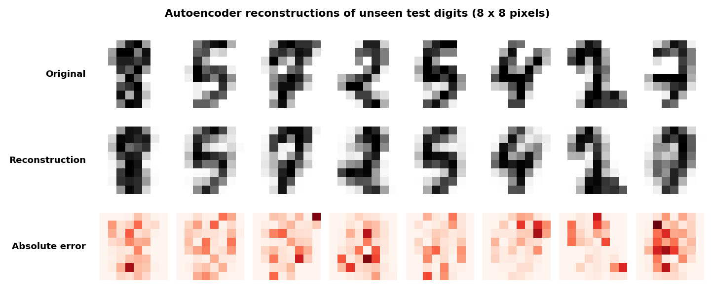
Each 64-pixel image has been squeezed into 8 numbers and rebuilt. The reconstructions are recognizable but softer than the originals. The error maps show that the loss concentrates along stroke edges, where fine detail is hardest to recover from a small code.

Latent Representations and Dimensionality Reduction

The 8-number code is a dimensionality reduction of the 64 pixel features, just as PCA with 8 components would be. A linear autoencoder (no activation functions) trained with mean squared error learns the same subspace as PCA. The advantage of a real autoencoder comes from its nonlinear activations, which allow it to represent curved structure that PCA cannot. The costs are training time, tuning, and no guarantee of a single unique solution.

You can use the code as input features for clustering such as K-means, for visualization, or for a downstream supervised model. To look at it, reduce the 8 dimensions to two with PCA, as the right panel of the next figure does.

Anomaly Detection With Autoencoders

The idea is simple. Train the autoencoder on normal data. It learns to reconstruct what it has seen. When it receives something different, it reconstructs poorly, so the reconstruction error rises. Flag inputs whose error exceeds a threshold.

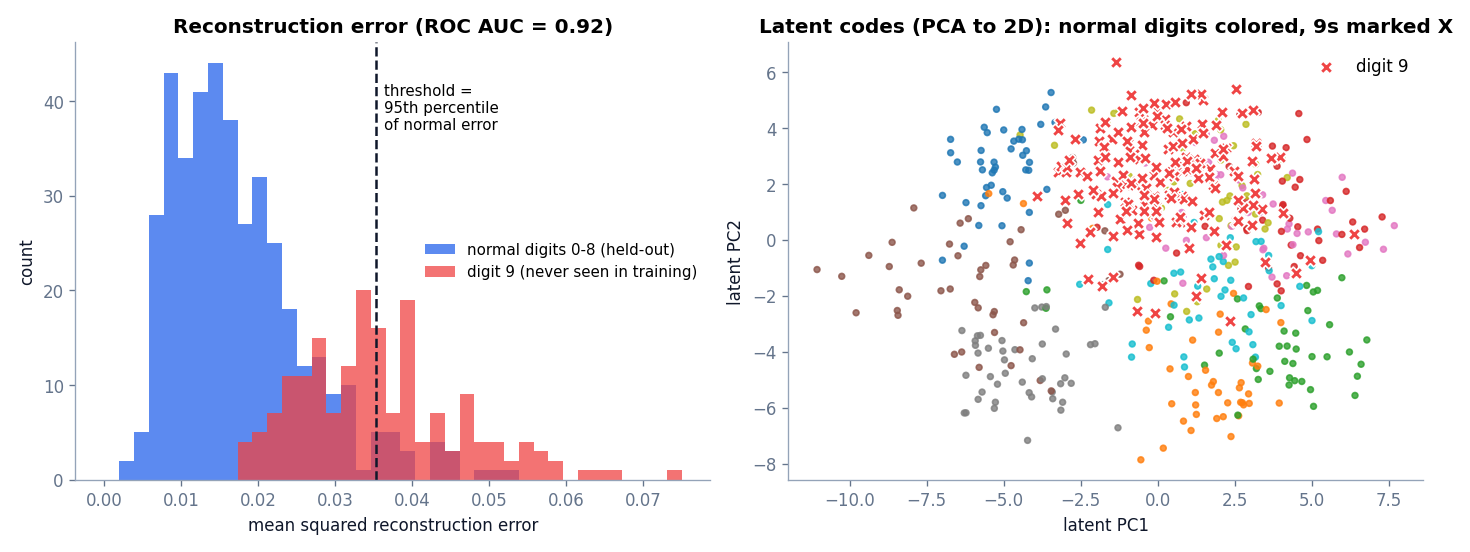
The script reports a threshold of 0.0353. Using it, 5.2 percent of held-out normal digits are flagged, which matches the 95th-percentile rule, and 46.7 percent of the digit 9 images are flagged. The ROC AUC, computed with the experiment’s labels purely for evaluation, is 0.916. That is a useful ranking signal, but it is far from perfect. More than half of the 9s fall below the threshold.

The reason is visible in the right panel: a handwritten 9 looks a lot like a 4, a 7, a 3, or a 0 at 8 by 8 resolution. An autoencoder that learned a general vocabulary of strokes can rebuild a 9 reasonably well, because it is made of strokes it knows. This is a well-known weakness. Autoencoders can generalize too well and reconstruct anomalies they were never meant to handle. Lowering the threshold catches more 9s at the cost of more false alarms. You can read the trade-off off the histogram.

For other anomaly detection methods and for discussion of evaluation, see Anomaly Detection in Machine Learning.

Autoencoder or PCA?

Fit PCA first. It takes seconds, needs no tuning, and gives a baseline reconstruction error for any chosen number of dimensions. Move to an autoencoder only if that baseline is not good enough and you have enough data to train a network, usually thousands of examples or more. If a PCA with eight components already reconstructs your data as well as the autoencoder does, the extra complexity is not paying for itself.

Design Choices and Variants

• Latent size. A smaller code compresses more and reconstructs worse. A larger code reconstructs better but may copy noise and anomalies. Treat it as a hyperparameter and validate it.
• Depth and width. Add layers for complex data such as photos. For small tabular data, one or two hidden layers are usually enough.
• Convolutional autoencoders use convolution layers and suit images.
• Denoising autoencoders corrupt the input and train the network to restore the clean version, which makes the code more robust.
• Variational autoencoders (VAEs) learn a probability distribution over the latent space and can generate new samples. They are a separate topic and beyond this introduction.

Limitations of Autoencoders

• They can reconstruct anomalies. As the digit 9 example shows, a flexible network may rebuild unfamiliar inputs well enough to evade detection.
• Training data must be mostly normal. If the training set contains many anomalies, the network learns to reconstruct them too.
• Reconstruction error is a proxy. A low error does not prove that the code is a good summary for another task.
• Tuning and compute. Choices such as learning rate, epochs, and architecture matter, and training can be unstable on some data.
• Loss of interpretability. The latent dimensions have no built-in meaning.
• Not always better than simpler methods. On small tabular data, PCA or Isolation Forest can match an autoencoder with far less effort. Try the simple baseline first.
• Thresholds need care. A percentile threshold flags a fixed share of normal data by construction. Pick it using validation data and the cost of false positives.

Common Mistakes

• Measuring reconstruction error only on the training set.
• Forgetting to scale inputs to the range the output activation can produce.
• Forgetting model.eval() and torch.no_grad() when scoring, which wastes memory and, for layers such as dropout, changes results.
• Making the bottleneck so large that the network learns the identity function.
• Claiming a detector works from a single run without checking different seeds.

Frequently Asked Questions

Is an autoencoder supervised or unsupervised?

It uses no external labels, since the input is the target, so it is considered unsupervised or self-supervised.

What is the latent space?

The latent space is the set of all possible codes the encoder can produce. Each input maps to a point in that lower-dimensional space.

What is the difference between PCA and an autoencoder?

PCA is a linear method with a closed-form solution. An autoencoder is a trained neural network that can learn nonlinear compression.

How does an autoencoder detect anomalies?

It is trained on normal data. Inputs that it reconstructs badly, meaning with high reconstruction error, are flagged as anomalies.

How big should the latent dimension be?

Start small relative to the input, for example one eighth to one quarter, and adjust using validation reconstruction error and downstream performance.

Conclusion

An autoencoder learns a compressed description of data by trying to rebuild it. The encoder produces a latent code, the decoder reconstructs the input, and the reconstruction loss drives the learning. The same trained network gives you a nonlinear dimensionality reduction and an anomaly score. Its main strengths are flexibility and the absence of labels. Its main risks are overly good reconstruction of anomalies, extra tuning, and the temptation to use it when a simpler method would do.

You have now seen the main unsupervised tools: clustering, dimensionality reduction, probabilistic models, anomaly detection, and neural representations. The final article combines them in a complete project. Continue with Unsupervised Learning Project: Customer Segmentation with Python.

References

• PyTorch documentation: torch.nn
• scikit-learn documentation: load_digits
• Hinton, G. E. and Salakhutdinov, R. R. (2006). Reducing the dimensionality of data with neural networks. Science, 313(5786), 504 to 507.
• Goodfellow, I., Bengio, Y., and Courville, A. (2016). Deep Learning, Chapter 14: Autoencoders. MIT Press.