
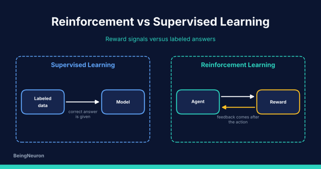
Reinforcement Learning vs Supervised Learning
Compare reinforcement learning vs supervised learning: how each learns, labels vs rewards, a comparison table, hybrid methods, and when to choose each.
Compare reinforcement learning vs supervised learning: how each learns, labels vs rewards, a comparison table, hybrid methods, and when to choose each.
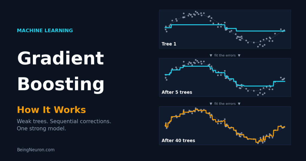
Learn how gradient boosting works: residuals, the loss gradient, learning rate and early stopping, with a hand-worked example, scikit-learn code for classification and regression, diagrams and real results.
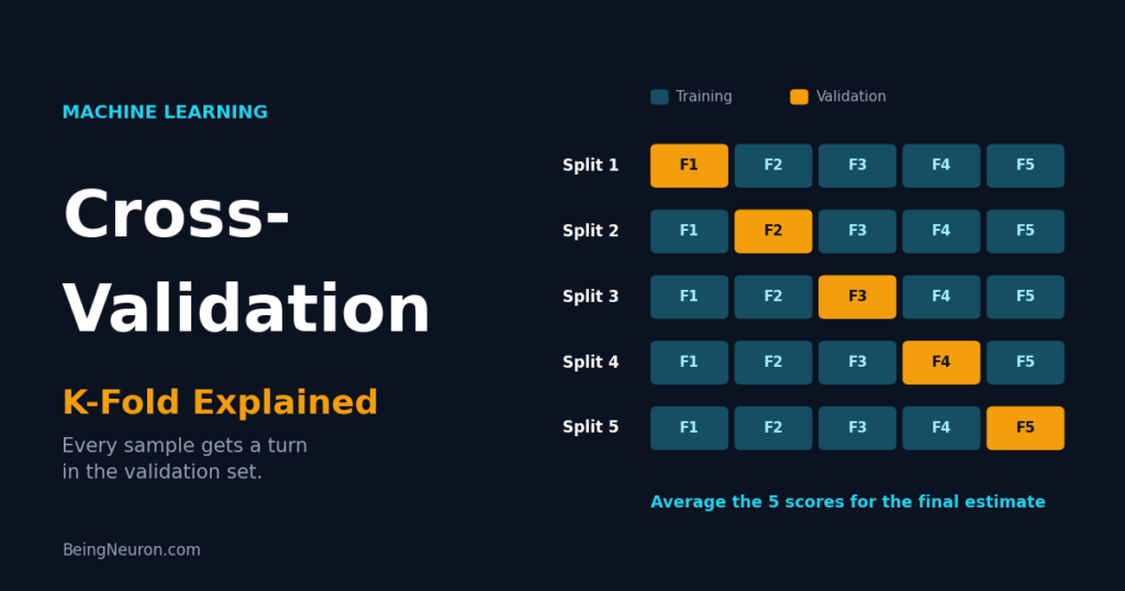
Learn how cross-validation and K-fold work in machine learning: choosing K, stratified, repeated, group and time-series splits, data leakage, and complete scikit-learn examples with real outputs.

Learn how Support Vector Machines (SVM) work: hyperplanes, margins, support vectors, the C parameter, and the kernel trick, with a complete scikit-learn tutorial, diagrams and measured results.
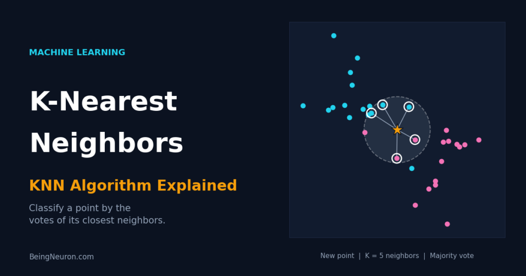
Understand how the K-Nearest Neighbors (KNN) algorithm works, how to choose k and a distance metric, and how to build and tune a KNN classifier in Python with scikit-learn, with diagrams and real results.
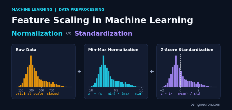
Learn how feature scaling works, when to use normalization (Min-Max) or standardization (Z-score), and how to apply both correctly in Python with scikit-learn, with worked examples, charts, and real results on the Wine dataset.
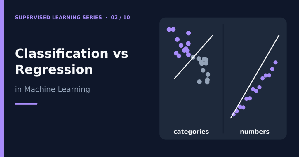
The difference between classification vs regression comes down to the answer you want. Classification predicts a category, such as “spam” or “not spam.” Regression predicts a number on a continuous scale, such as a house price or tomorrow’s temperature. Both belong to supervised learning, so both learn from labeled examples. This guide explains how the two tasks differ, which algorithms and metrics fit each one, and how to decide which task your own problem needs. If you are new to the field, read What Is Supervised Learning? first. Table of contents Classification vs regression at a glance What is classification? What is regression? Common algorithms for each task Evaluation metrics for each task How to choose the right task A side-by-side Python example Common mistakes Frequently asked questions Conclusion Classification vs regression at a glance The table below summarizes the main differences. The rows give you a quick reference, and the sections after it explain each point. Aspect Classification Regression Goal Assign an example to a class Predict a numeric quantity Output type Discrete labels (for example “cat,” “dog”) Continuous numbers (for example 245.7) Typical question “Which one?” or “Yes or no?” “How much?” or “How many?” Example Will this customer cancel? (yes/no) How much will this customer spend? Common algorithms Logistic regression, decision tree classifier, k-nearest neighbors Linear regression, decision tree regressor, random forest regressor Common metrics Accuracy, precision, recall, F1-score, ROC-AUC MAE, MSE, RMSE, R-squared Typical diagnostic Confusion matrix Predicted-versus-actual plot, residual plot One rule sits behind every row: the target variable decides the task, not the algorithm. If the target is a category, you have a classification problem. If the target is a measurable number, you have a regression problem. What is classification? Classification models learn to place each example into one of several predefined classes. The model looks at the features, such as the words in an email, and outputs a class label. Binary classification Binary classification has exactly two classes. Examples include spam versus not spam, fraud versus legitimate, and disease present versus absent. By convention, programmers often call one class “positive” and the other “negative.” The positive class is usually the one you care most about finding. Multiclass classification Multiclass classification has three or more classes, and each example belongs to exactly one. Recognizing handwritten digits from 0 to 9 and sorting news stories into sports, politics, or business are typical cases. Multilabel classification In multilabel classification, one example can have several labels at once. A photo might be tagged “beach,” “sunset,” and “people” together. Many beginners overlook this type, but it appears often in tagging systems. Many classifiers can output probabilities, for example “82% likely to be spam,” and then convert the probability into a class using a threshold. This detail causes a lot of confusion, because a probability is a number. The model is still a classifier, since its final job is to choose a class. What is regression? Regression models predict a numeric value. The target can take any value in a range, and nearby values mean similar things: a price of 200,000 is close to 201,000. The model outputs one number for each example. Typical regression tasks include predicting house prices, estimating how many minutes a delivery will take, forecasting energy use, and predicting a patient’s blood pressure from other measurements. A regression model rarely hits the exact true value, so we judge it by how far off its predictions are on average. The simplest version, simple linear regression, fits a straight line through the data. You can study it in detail in Linear Regression Explained with Examples. Common algorithms for each task Many algorithms come in two versions: one for classification and one for regression. The core idea stays the same, but the final output and the loss function differ. Algorithm family Classification version Regression version Linear models Logistic regression Linear regression, ridge, lasso Decision trees DecisionTreeClassifier DecisionTreeRegressor Random forests RandomForestClassifier RandomForestRegressor Nearest neighbors KNeighborsClassifier KNeighborsRegressor Support vector machines SVC SVR Logistic regression deserves a special note. Despite its name, it is a classification algorithm. It uses a regression-style equation internally, then converts the result into a probability and a class. The article on logistic regression explains how this works. Decision trees show the “two versions” idea clearly. A classification tree ends each branch with a class label. A regression tree ends each branch with an average of the numbers that landed there. You can explore the method in Decision Trees in Machine Learning: How They Work. Evaluation metrics for each task You cannot use the same score for both tasks. Accuracy means nothing when the target is a price, and average error means nothing when the target is a class. Classification metrics Accuracy: the share of predictions that are correct. Precision: among examples predicted positive, the share that really are positive. Recall: among truly positive examples, the share the model found. F1-score: a single number that balances precision and recall. ROC-AUC: how well the model ranks positives above negatives across all thresholds. Regression metrics MAE (mean absolute error): the average size of the errors, in the units of the target. MSE (mean squared error): the average of squared errors, which punishes large mistakes more. RMSE (root mean squared error): the square root of MSE, back in the units of the target. R-squared: the share of the target’s variation that the model explains. Each metric has traps. For example, accuracy can look excellent on a dataset where 95% of examples belong to one class. The full discussion lives in How to Evaluate a Supervised Learning Model. How to choose the right task Use these questions to decide. Work through them in order. Step 1: Look at the target Ask what the answer looks like. If it is a label from a list, choose classification. If it is a quantity that can take many values, choose regression. Step 2: Think about what the decision needs Sometimes the same business question can be framed both ways. A store might want
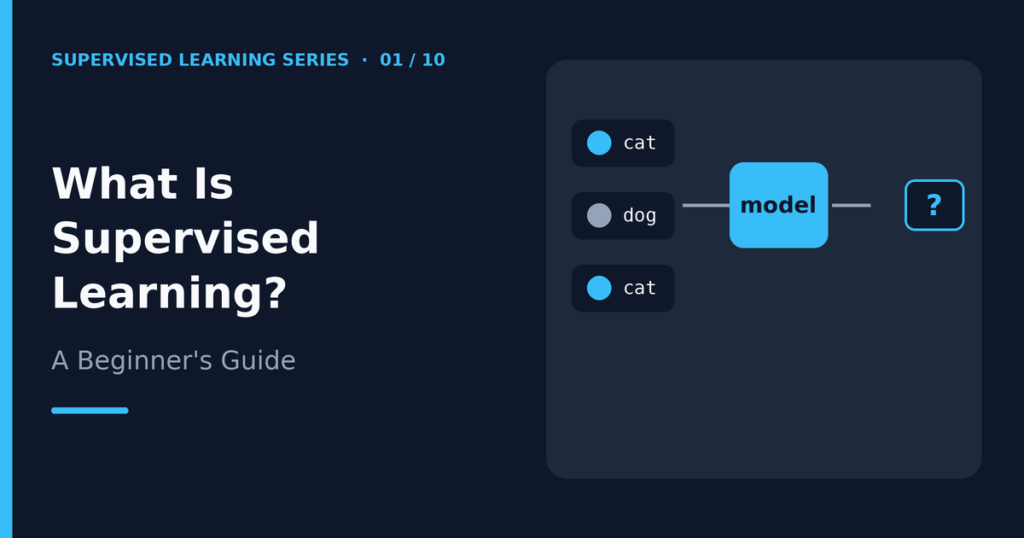
Supervised learning is a type of machine learning where a model learns from examples that already include the correct answer. You show the model many inputs together with their known outputs. The model finds the pattern that connects them, and then it uses that pattern to make predictions on new data it has never seen. That is the short answer to “what is supervised learning?” This guide expands on it in plain English. You will learn the key terms, see how training and prediction work, run a small Python example, and understand where supervised learning works well and where it struggles. Table of contents What is supervised learning? The key terms you need to know How supervised learning works step by step A simple supervised learning example The two main types of supervised learning Common applications Advantages and limitations Supervised vs unsupervised learning Where to go next Frequently asked questions Conclusion What is supervised learning? Think about how a child learns to recognize fruit. A parent points at an apple and says “apple.” Later the parent points at a banana and says “banana.” After enough examples, the child can name a fruit they have never seen in that exact shape or color. The parent acts as the supervisor, because the parent supplies the right answer for every example. Supervised learning works the same way. The “supervisor” is the labeled dataset. Each row of data comes with the answer the model should learn to produce. The algorithm studies thousands of these pairs and adjusts itself until its own guesses match the known answers as closely as possible. The real goal is not to memorize the examples. The goal is generalization: making good predictions on new data. Everything else in supervised learning, from splitting your data to choosing a metric, exists to check whether the model generalizes. The key terms you need to know Four terms appear in almost every supervised learning tutorial. Learn them once and the rest of the topic becomes much easier to read. Labeled dataset A labeled dataset is a table in which every example includes the correct answer. In a spam filter, each email is an example, and its label is “spam” or “not spam.” People often create labels by hand, collect them from past records, or measure them with sensors. Good labels matter a great deal, because the model learns whatever the labels teach it, including mistakes. Features Features are the input columns that describe each example. For a house, the features might be size, number of bedrooms, and neighborhood. For an email, they might be the number of links, certain words, and the sender’s domain. You may also see features called inputs, predictors, or independent variables. Programmers usually write the feature table as X. Target variable The target variable is the answer you want the model to predict. It is also called the label, the output, or the dependent variable. In the house example, the target is the sale price. Programmers usually write it as y. Model and parameters The model is the mathematical function that turns features into a prediction. It contains internal numbers called parameters (also called weights). Training means finding parameter values that make the predictions match the labels well. How supervised learning works step by step Most supervised learning projects follow the same basic path. The details change from one algorithm to another, but the outline stays the same. Step 1: Collect and prepare labeled data You gather examples and make sure each one has a label. You also clean the data, handle missing values, and convert text categories into numbers when the algorithm requires it. Step 2: Split the data You set aside part of the data before training starts. The model trains on the larger part, called the training set. You keep the smaller part, called the test set, hidden until the end. The article on training data vs testing data explains this split in detail. Step 3: Train the model During training, the algorithm makes predictions on the training examples and compares them with the true labels. A loss function measures how wrong the predictions are. The algorithm then adjusts its parameters to reduce that loss. It repeats this cycle many times, or it solves for the best parameters in one calculation, depending on the method. Step 4: Make predictions After training, you give the model features from new examples, and it returns predicted targets. In scikit-learn, this is the predict() method. The model does not see the true answers at this stage. Step 5: Evaluate and improve You compare the predictions on the test set with the real labels and calculate a metric such as accuracy or error. If performance is poor, you can try better features, a different algorithm, or different settings. The guide to supervised learning model evaluation covers the metrics in depth. A simple supervised learning example Here is a tiny example you can run yourself. Suppose a teacher records how many hours eight students studied and slept, and whether each student passed. The two numbers are the features. Passing is the target: 1 means passed and 0 means failed. from sklearn.neighbors import KNeighborsClassifier # Features: [hours_studied, hours_slept]; target: 1 = passed, 0 = failed X = [[1, 5], [2, 6], [3, 5], [4, 7], [6, 6], [7, 8], [8, 7], [9, 6]] y = [0, 0, 0, 0, 1, 1, 1, 1] model = KNeighborsClassifier(n_neighbors=3) model.fit(X, y) # training print(model.predict([[5, 7], [2, 5]])) # prediction on new students The code uses the k-nearest neighbors algorithm, one of the simplest supervised methods. The fit() call trains the model. The predict() call looks at each new student, finds the three most similar students in the training data, and lets them vote. When I ran this code, it printed: [1 0] The model predicts that the student who studied 5 hours and slept 7 hours will pass, and that the student who studied 2 hours and slept 5 hours will fail. Eight rows are far
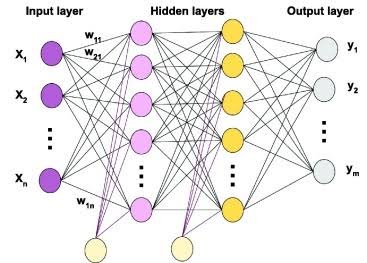
A Multilayer Perceptron (MLP) is one of the fundamental architectures in artificial neural networks and deep learning. It uses multiple layers of interconnected neurons to learn patterns from data and make predictions. A basic perceptron can only solve linearly separable problems. A multilayer perceptron overcomes this limitation by adding hidden layers and non-linear activation functions. As a result, an MLP can learn much more complex relationships. MLPs form an important foundation for understanding neural networks. Concepts such as weights, biases, activation functions, forward propagation, loss functions, backpropagation, and gradient-based optimization all play a central role in how they work. This guide explains what a multilayer perceptron is, how its architecture works, the formulas behind it, why non-linearity matters, how an MLP solves the XOR problem, how to calculate its parameters, and how to build one in Python. What Is a Multilayer Perceptron? A Multilayer Perceptron (MLP) is a type of feedforward artificial neural network that contains an input layer, one or more hidden layers, and an output layer. The network receives input data, transforms that data through its hidden layers, and produces a prediction through its output layer. A typical MLP follows this structure: Input Layer → Hidden Layer(s) → Output Layer Each neuron receives information from the previous layer, applies weights and biases, performs a mathematical calculation, and passes the result through an activation function. During training, the MLP adjusts its weights and biases to reduce prediction errors. MLPs can perform both: Classification Regression For example, an MLP can classify whether an email is spam or predict the price of a house. Multilayer Perceptron Architecture A standard multilayer perceptron contains three main types of layers. Input Layer The input layer receives the original data. Each input neuron usually represents one feature. For example, a model that predicts student performance might receive: Hours studied Attendance percentage Previous exam score Number of completed assignments If the dataset contains four input features, the input layer usually receives four input values. The input layer does not perform the main learning process. Instead, it passes the feature values to the first hidden layer. Hidden Layers Hidden layers perform most of the transformations inside an MLP. Each neuron receives outputs from the previous layer, calculates a weighted sum, adds a bias, and applies an activation function. An MLP can contain: One hidden layer Several hidden layers Adding hidden layers allows the network to build increasingly complex representations of the input data. For example, an early hidden layer may learn simple relationships, while later layers can combine those relationships into more complex patterns. Output Layer The output layer produces the final prediction. The number of output neurons and the activation function depend on the problem. For example: A regression problem may use one output neuron. A binary classification problem often uses one output neuron with a sigmoid function. A multi-class classification problem often uses multiple output neurons with softmax. Are MLP Layers Fully Connected? Yes. A standard multilayer perceptron uses fully connected layers, also called dense layers. In a fully connected layer, every neuron in one layer connects to every neuron in the next layer. For example, if an input layer contains four neurons and the next hidden layer contains six neurons, every one of the four inputs connects to all six hidden neurons. These connections contain learnable weights. This fully connected structure gives an MLP its ability to combine information from multiple input features. However, it can also create a large number of parameters as the network grows. Multilayer Perceptron Formula The mathematical foundation of an MLP begins with the calculation performed by a single neuron. A neuron calculates a weighted sum: [ z = w_1x_1 + w_2x_2 + \dots + w_nx_n + b ] The neuron then applies an activation function: [ a = f(z) ] Where: (x_1, x_2, \dots, x_n) are the input values (w_1, w_2, \dots, w_n) are the weights (b) is the bias (z) is the weighted input (f) is the activation function (a) is the output of the neuron An MLP performs this calculation across many neurons and layers. General Multilayer Perceptron Formula For any layer (l), an MLP calculates the weighted input as: \mathbf{W}^{(l)} \mathbf{A}^{(l-1)} + \mathbf{b}^{(l)} ] The layer then applies an activation function: f\left( \mathbf{Z}^{(l)} \right) ] Combining both steps gives the general MLP formula: f\left( \mathbf{W}^{(l)} \mathbf{A}^{(l-1)} + \mathbf{b}^{(l)} \right) ] Where: (\mathbf{A}^{(l-1)}) is the output from the previous layer (\mathbf{W}^{(l)}) is the weight matrix (\mathbf{b}^{(l)}) is the bias vector (\mathbf{Z}^{(l)}) is the weighted input (f) is the activation function (\mathbf{A}^{(l)}) is the output of the current layer The output from one layer becomes the input to the next layer. MLP Formula for Multiple Layers Consider an MLP with an input layer, two hidden layers, and an output layer. The original input is: [ \mathbf{A}^{(0)} = \mathbf{X} ] First Hidden Layer The first hidden layer calculates: \mathbf{W}^{(1)} \mathbf{X} + \mathbf{b}^{(1)} ] It then applies an activation function: f_1 \left( \mathbf{W}^{(1)} \mathbf{X} + \mathbf{b}^{(1)} \right) ] Second Hidden Layer The second hidden layer receives the output from the first hidden layer: \mathbf{W}^{(2)} \mathbf{A}^{(1)} + \mathbf{b}^{(2)} ] Its output becomes: f_2 \left( \mathbf{W}^{(2)} \mathbf{A}^{(1)} + \mathbf{b}^{(2)} \right) ] Output Layer The output layer receives the final hidden representation: \mathbf{W}^{(L)} \mathbf{A}^{(L-1)} + \mathbf{b}^{(L)} ] The network then produces the prediction: f_L \left( \mathbf{W}^{(L)} \mathbf{A}^{(L-1)} + \mathbf{b}^{(L)} \right) ] Here, (\hat{\mathbf{Y}}) represents the predicted output. Understanding Matrix Dimensions in an MLP Understanding matrix dimensions helps explain how an MLP processes multiple inputs and neurons efficiently. Suppose: The input contains (n) features. The first hidden layer contains (h) neurons. The input vector can have the shape: [ \mathbf{X} \in \mathbb{R}^{n} ] The weight matrix can have the shape: [ \mathbf{W}^{(1)} \in \mathbb{R}^{h \times n} ] The bias vector can have the shape: [ \mathbf{b}^{(1)} \in \mathbb{R}^{h} ] The output of the hidden layer therefore has the shape: [ \mathbf{A}^{(1)} \in \mathbb{R}^{h} ] For a batch of (m) examples, implementations may organize the dimensions differently depending on the framework. However, the