
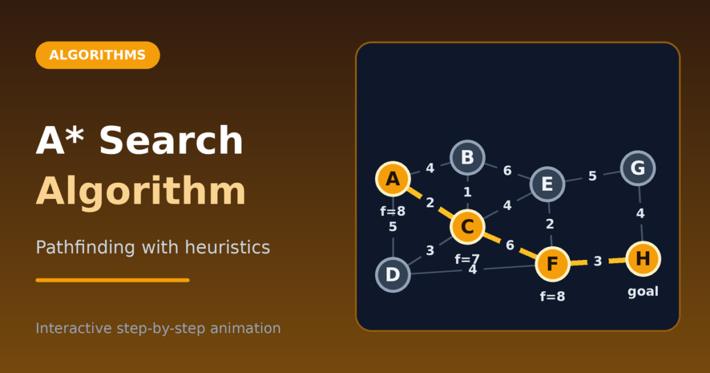
A* Search Algorithm
Learn the A* search algorithm with an interactive pathfinding visualization, step-by-step example, heuristics, pseudocode, JavaScript code, and complexity.
Learn the A* search algorithm with an interactive pathfinding visualization, step-by-step example, heuristics, pseudocode, JavaScript code, and complexity.

Understand the bubble sort algorithm with an interactive visualization, step-by-step example, pseudocode, JavaScript code, and complexity analysis.
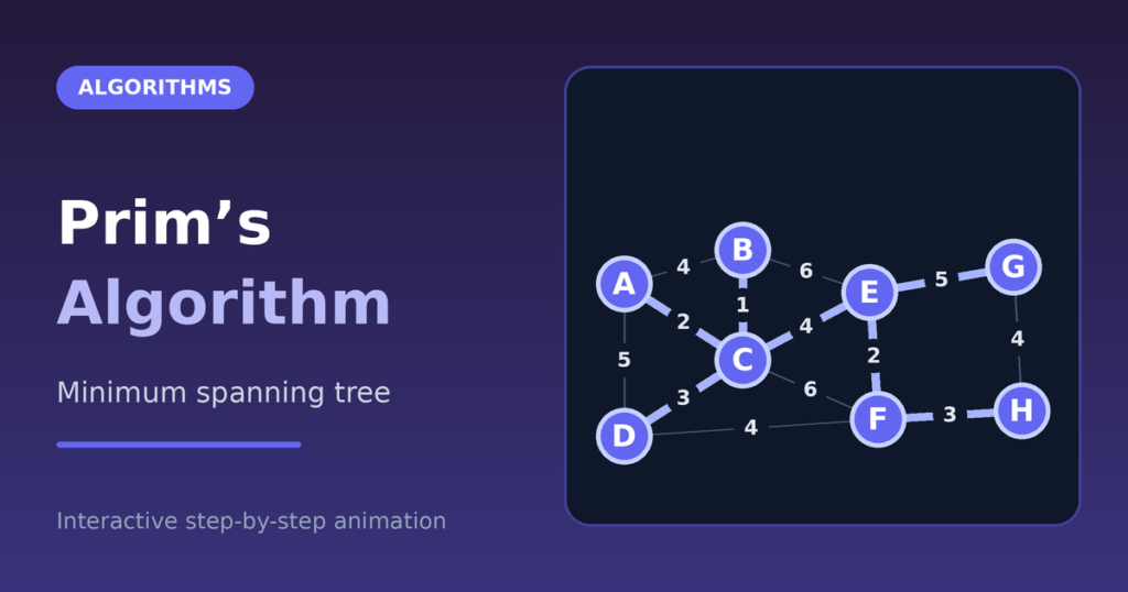
Learn Prim’s algorithm for minimum spanning trees with an interactive visualization, step-by-step example, pseudocode, JavaScript code, and complexity.
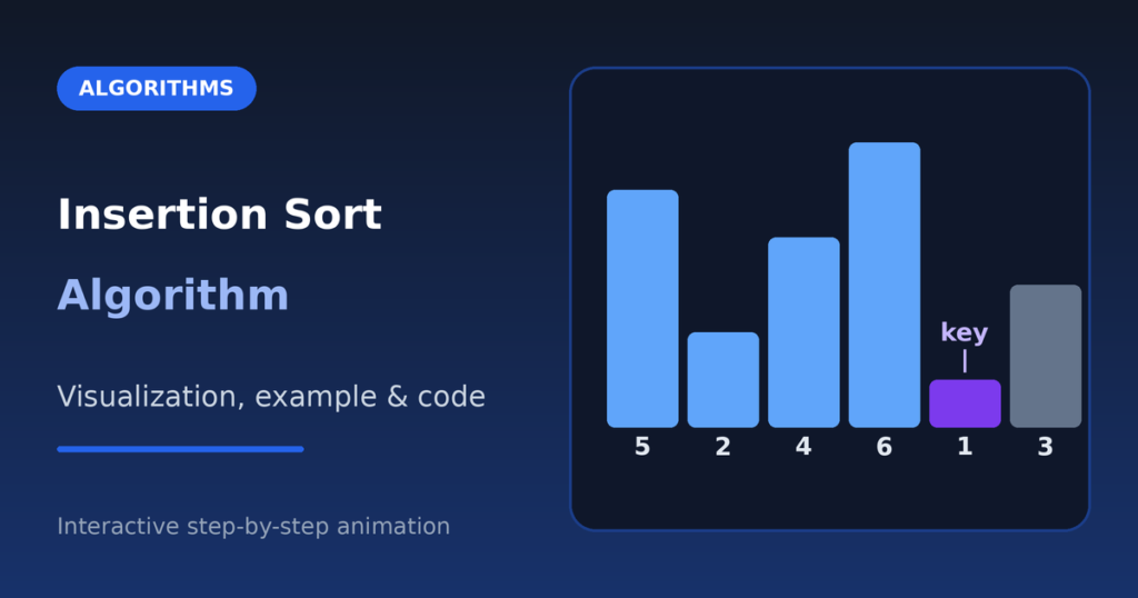
Learn the insertion sort algorithm with an interactive step-by-step visualization, example, pseudocode, JavaScript code, and time and space complexity.
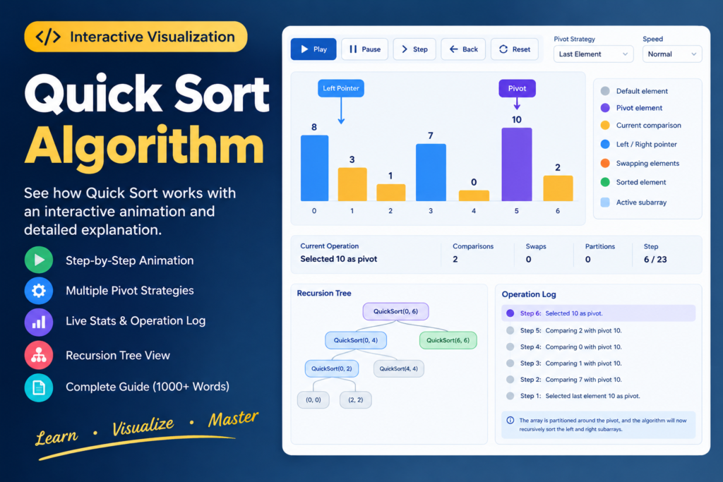
The Quick Sort algorithm sorts an array by picking a pivot, partitioning the other items around it, and repeating on the smaller parts. Use the visualization below to run it, pause it, step through it, and even step backward. ▶ Play⏮ BackStep ⏭↺ ResetRun to completionShuffle SpeedVery SlowSlowNormalFastVery Fast PivotLast elementFirst elementMiddle elementRandom element Size (5–60) Min Max Generate new array Apply arrayUnsortedP = pivot? = compared⇄ = swapped✓ = final positioni = partition boundaryactive subarray Operation log Recursive calls Complexity (theory): best O(n log n), average O(n log n), worst O(n²). Extra space: O(log n) stack when balanced, O(n) worst case. In-place partitioning, usually not stable. Real behavior depends on pivot choice, input and implementation. The counters above are measured for your array only. Introduction to Quick Sort Quick Sort is a comparison-based sorting algorithm and one of the best-known divide and conquer algorithms. Developers use it because it is simple, sorts in place, and is fast on many real inputs. Its key idea is partitioning: rearrange items so the pivot lands in its final position, with items that belong before it on one side and items that belong after it on the other. Learning Quick Sort is a great way to understand sorting algorithms and recursion. What Is the Quick Sort Algorithm? The Quick Sort algorithm sorts an array by choosing one element, the pivot, and partitioning the rest around it. After partitioning, the pivot never moves again. Quick Sort then sorts the left part and the right part the same way. Take [3, 1, 2]. With pivot 2, the value 1 goes left and 3 stays right, giving [1, 2, 3]. Each step shrinks the problem until pieces are too small to need sorting. How Quick Sort Works Step by Step Choose a pivot. Partition the array around the pivot. Recursively sort the left subarray. Recursively sort the right subarray. Finish when each subarray has zero or one element. The exact moves in step 2 depend on the partition scheme. This page uses the Lomuto scheme for every pivot strategy: the chosen pivot is first swapped to the end of the subarray, then partitioned. Its invariant: while scanning, items from the start up to boundary i hold values less than or equal to the pivot, and items from i up to the scan position hold values greater than the pivot. Because of the “less than or equal” rule, equal values may sit on the left, so do not assume everything on the left is strictly smaller. Understanding the Pivot in Quick Sort The pivot is the reference value for a partition. Pivot choice matters because it decides how even the two parts are. Common strategies: First element: easy, but slow on already sorted input. Last element: also easy and equally weak on sorted input. Middle element: handles sorted and reverse-sorted arrays well. Note that the middle index is not the median value. Random element: makes consistently bad splits unlikely. Median of three (optional): use the median of the first, middle and last values for better balance. Try each strategy in the visualization on a sorted array and compare the comparison counts. Quick Sort Example With a Step-by-Step Walkthrough Array [8, 3, 1, 7, 0, 10, 2], Lomuto partition, last element as pivot. Pivot is 2, boundary i = 0. Scan: 8 and 3 are greater than 2, so nothing moves. 1 is at most 2, so swap it with index 0: [1, 3, 8, 7, 0, 10, 2], i = 1. 7 is greater. 0 is at most 2, so swap with index 1: [1, 0, 8, 7, 3, 10, 2], i = 2. 10 is greater. Place the pivot: swap index 2 with the end: [1, 0, 2, 7, 3, 10, 8]. The 2 is final. Left part [1, 0], pivot 0: nothing is smaller, so swap 1 and 0 to get [0, 1]. Right part [7, 3, 10, 8], pivot 8: 7 and 3 stay in the left group, 10 is greater, then swap 10 and 8: [7, 3, 8, 10]. Sort [7, 3] with pivot 3: swap to [3, 7]. The final array is [0, 1, 2, 3, 7, 8, 10]. Quick Sort Pseudocode quickSort(A, lo, hi): if lo >= hi: return // base case p = partition(A, lo, hi) quickSort(A, lo, p – 1) quickSort(A, p + 1, hi) partition(A, lo, hi): // pivot = A[hi] i = lo for j = lo to hi – 1: if A[j] <= A[hi]: swap A[i], A[j]; i = i + 1 swap A[i], A[hi] return i // pivot’s final index The base case stops recursion on zero or one element. The partition function returns the pivot’s final index, which the recursive calls use to exclude it. Quick Sort Implementation in JavaScript function quickSort(input) { const a = […input]; // copy: input is not modified const sort = (lo, hi) => { if (lo >= hi) return; // handles [] and [x] const p = partition(lo, hi); sort(lo, p – 1); sort(p + 1, hi); }; const partition = (lo, hi) => { const pivot = a[hi]; let i = lo; for (let j = lo; j < hi; j++) { if (a[j] <= pivot) { [a[i], a[j]] = [a[j], a[i]]; i++; } } [a[i], a[hi]] = [a[hi], a[i]]; return i; }; sort(0, a.length – 1); return a; } The function copies the input, so the original stays unchanged. The partition loop moves small values to the left of boundary i, and the final swap puts the pivot in place. For other pivot strategies, swap the chosen element to index hi first. Time Complexity of Quick Sort Quick Sort time complexity depends on partition balance. When partitions are roughly even, there are about log n levels and each level does O(n) work, so time is O(n log n). If every partition is extremely lopsided, such as a sorted array with a first or last pivot, there are n levels and the time grows
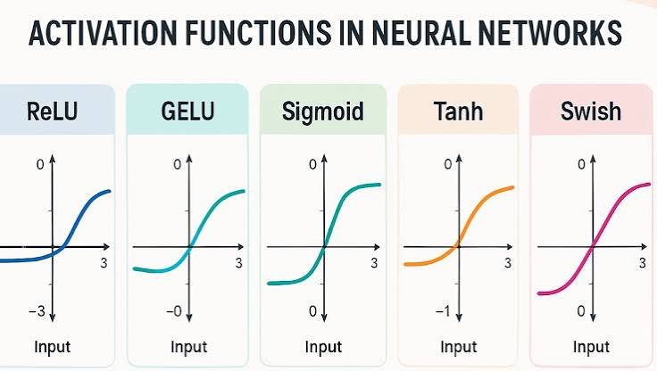
What Is an Activation Function? An activation function is a mathematical function that helps a neural network learn patterns from data. It takes a neuron’s calculated value as input and transforms that value into an output. Neural networks use activation functions to learn complex relationships between inputs and outputs. Without them, even a neural network with many layers would behave like a single linear model if every layer only performed a linear operation. For example, imagine you want to build a neural network that identifies cats and dogs in images. The network must learn patterns such as edges, shapes, ears, eyes, and fur. An activation function helps the network learn these complex patterns by introducing nonlinearity into its calculations. Different activation functions serve different purposes. Some work well in hidden layers, while others help the network produce probabilities for classification tasks. In this guide, you will learn how activation functions work, explore the most common types, compare their advantages and disadvantages, and understand how to choose the right one for a neural network. How Does an Activation Function Work? A neural network neuron receives input values, multiplies them by weights, adds a bias, and calculates a result. The neuron then passes this result through an activation function. A neuron typically calculates its output using two steps. Step 1: Calculate the weighted sum [ z = w_1x_1 + w_2x_2 + b ] Here: (x_1) and (x_2) represent input values. (w_1) and (w_2) represent weights. (b) represents the bias. (z) represents the weighted sum before activation. Step 2: Apply the activation function [ a = f(z) ] In this equation, (f) represents the activation function, and (a) represents the neuron’s output. Let’s use an example. Suppose a neuron calculates a weighted sum of 2. If the network uses the ReLU activation function, the neuron produces an output of 2. If the weighted sum equals -2, ReLU produces 0. This behavior allows the network to respond differently to different inputs. Why Do Neural Networks Need Activation Functions? Activation functions play an important role in neural network learning. They provide several benefits. 1. They introduce nonlinearity Real-world problems rarely follow simple linear relationships. Image recognition, speech processing, language understanding, and fraud detection all involve complex patterns. Activation functions allow neural networks to learn these nonlinear relationships. Without nonlinear activation functions, stacking multiple layers would not give a network the full learning power of a deep neural network. 2. They help neural networks learn complex patterns A neural network can combine the outputs of many neurons to identify increasingly complex features. Earlier layers may detect simple patterns, while deeper layers combine those patterns into more meaningful representations. Activation functions help the network build these representations during training. 3. They support different prediction tasks Different activation functions produce different output ranges. For example, sigmoid produces values between 0 and 1, which makes it useful for binary classification. Softmax converts a vector of scores into a probability distribution across multiple classes. The choice of activation function affects how the network learns and how it represents its predictions. Types of Activation Functions in Neural Networks Researchers and developers use several activation functions when building neural networks. The most common choices include ReLU, sigmoid, tanh, softmax, and newer functions such as GELU and Leaky ReLU. 1. ReLU Activation Function The ReLU activation function, which stands for Rectified Linear Unit, is one of the most widely used activation functions in deep learning. It returns the input value when the input is positive and returns zero when the input is negative. Its mathematical formula is: [ f(x) = \max(0,x) ] For example: If (x = 5), ReLU returns 5. If (x = 0), ReLU returns 0. If (x = -3), ReLU returns 0. ReLU has a simple calculation, which makes it computationally efficient. It also helps reduce the vanishing gradient problem for positive inputs compared with sigmoid and tanh. Advantages of ReLU It is simple and fast to calculate. It works well in many deep neural networks. It helps maintain stronger gradients for positive inputs. It often provides effective training performance in hidden layers. Disadvantages of ReLU ReLU can suffer from the dying ReLU problem. If a neuron repeatedly receives negative inputs, it may produce zero and stop learning through its usual gradient. This can make the neuron inactive during training. When should you use ReLU? Use ReLU as a starting choice for hidden layers in many feedforward neural networks and convolutional neural networks. Test alternatives when training performance or gradient behavior becomes a problem. 2. Sigmoid Activation Function The sigmoid activation function converts any real-valued input into a number between 0 and 1. Its formula is: [ f(x) = \frac{1}{1+e^{-x}} ] For example, sigmoid produces approximately 0.5 when the input equals zero. Large positive inputs produce values close to 1, while large negative inputs produce values close to 0. This output range makes sigmoid useful when a model needs to predict the probability of a binary outcome. Imagine a model that predicts whether an email is spam. It might produce a sigmoid output of 0.92, which indicates a predicted spam probability of 92%. Advantages of sigmoid It produces outputs between 0 and 1. It works well as an output activation for binary classification. It converts a single score into a probability-like value. Disadvantages of sigmoid Sigmoid can cause the vanishing gradient problem when its inputs become very positive or very negative. Its outputs can also make optimization slower in deep networks. When should you use sigmoid? Use sigmoid in the output layer of a binary classification model when you want one probability for a positive class. For training, developers commonly combine it with binary cross-entropy loss, often using a numerically stable implementation that accepts logits directly. 3. Tanh Activation Function The tanh activation function, also called the hyperbolic tangent function, maps input values to a range between -1 and 1. Its formula is: [ f(x) = \tanh(x) ] Tanh produces zero when the input equals zero. Positive inputs produce

Binary Searh Tree Visualization Learning data structures can feel difficult when you only read code and theory. Binary search tree visualization makes the process easier by turning abstract operations into something you can see. Instead of imagining how nodes connect, you can watch a tree grow as you insert values. You can also see how searching, deletion, and traversal work step by step. This makes BSTs easier to understand for students, self taught programmers, and software engineering candidates preparing for interviews. What Is a Binary Search Tree? A binary search tree (BST) is a tree based data structure that stores values in an organized way. Each element sits inside a node, which can connect to up to two other nodes. The top node is called the root. The nodes connected below it are called children. The child on the left is the left child, while the child on the right is the right child. A BST follows one important ordering rule: Values smaller than a node go to its left. Values larger than a node go to its right. Duplicate values depend on the rules used by the particular implementation. For example, suppose you insert: 50, 30, 70, 20, 40, 60, 80 The resulting tree looks like this: 50 / \ 30 70 / \ / \ 20 40 60 80 This structure makes searching more efficient when the tree stays reasonably balanced. Why Binary Search Tree Visualization Matters Reading a BST implementation can tell you what the algorithm does. However, a visual representation helps you understand why it works. A binary tree visualization shows relationships between nodes directly. You can see which node acts as the root, where each child connects, and how the tree changes after every operation. Visualization also helps you understand recursion. For example, when searching for 40, you start at 50. Since 40 is smaller, you move left to 30. Since 40 is larger than 30, you move right and find the value. A visualizer can highlight this path as the algorithm runs. It also makes time complexity easier to understand: Balanced BST: Search can take about O(log n). Unbalanced BST: Search can degrade to O(n). Insertion: Usually O(log n) in a balanced tree. Deletion: Usually O(log n) in a balanced tree. This difference becomes much clearer when you watch a tree become balanced or turn into a long chain. How a Binary Tree Visualizer Works A binary tree visualizer converts the logical structure of a tree into a visual diagram. Most interactive tools let you enter values and watch the application create nodes and edges. A typical visualizer can support: Inserting values. Searching for values. Deleting nodes. Animating tree traversal. Highlighting comparisons and paths. Showing the tree after each operation. A good binary tree visualizer should let you control the animation. Step by step controls are especially useful because they let you pause after each comparison. Insertion Animation When you insert a value, the algorithm starts at the root. Suppose the tree contains 50 and you insert 30. The algorithm compares 30 with 50. Since 30 is smaller, it moves left. If that position is empty, it creates a new node there. Now suppose you insert 70. Compare 70 with 50. Since 70 is larger, move right. Create the node in the empty position. A binary search tree visualizer can animate each comparison and movement. This helps you connect the code with the actual tree structure. Deletion and Rebalancing Deletion can feel more complicated because the algorithm handles three main cases. Case 1: Leaf node A leaf has no children. The algorithm can simply remove it. Case 2: One child If a node has one child, the algorithm connects that child to the node’s parent. Case 3: Two children If a node has two children, the algorithm usually replaces its value with a suitable value from its subtree. A common choice is the smallest value in the right subtree, known as the in order successor. A visualizer can show these connections changing during deletion. Note that a basic BST does not automatically rebalance itself. Balanced structures such as AVL trees and Red Black trees use additional rules to maintain better height. Traversal Animation: In-order, Pre-order, Post-order Traversal means visiting the nodes of a tree according to a specific order. The three common depth first traversals are: In-order: Left → Root → Right Pre-order: Root → Left → Right Post-order: Left → Right → Root In-order traversal has a special property in a BST. It visits values in sorted order. For the tree above: In-order: 20, 30, 40, 50, 60, 70, 80 Pre-order: 50, 30, 20, 40, 70, 60, 80 Post-order: 20, 40, 30, 60, 80, 70, 50 A visualizer can highlight each node as the traversal moves through the tree. This makes recursion and traversal order much easier to remember. Best Binary Search Tree Visualizer Tools Online When looking for a binary search tree visualization online, focus on features rather than a tool’s name. A useful visualizer should provide: Interactive node insertion. Search and deletion operations. Step by step animation. Traversal visualization. Clear node and edge labels. Controls for pausing and restarting. Support for duplicate values or clear duplicate rules. Mobile friendly design. Accessible controls. Open source code if you want to study the implementation. You should also test unusual inputs. Try inserting sorted values such as 10, 20, 30, 40, 50. This quickly shows how a BST can become heavily unbalanced. Binary Search Tree Visualization Online vs. Building Your Own Using an online visualizer is usually the fastest way to understand BST operations. You can focus on the data structure without spending time building the interface. Building your own visualizer offers a different benefit. It forces you to understand both the algorithm and the visual representation. For example, you could build a simple project using: Python + Matplotlib for basic diagrams. JavaScript + D3.js for interactive browser visualizations. HTML and CSS for the interface. JavaScript animations for step by step operations. A
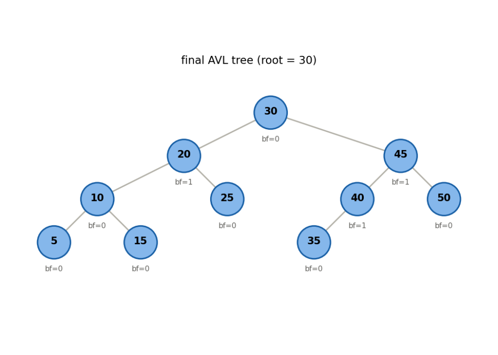
Avl Tree Visualization An AVL Tree is a special type of Binary Search Tree that automatically keeps itself balanced. A normal Binary Search Tree can provide very fast searching, insertion, and deletion when the tree remains balanced. In that situation, these operations can take O(log n) time. However, a normal Binary Search Tree does not automatically control its shape. If we insert values in a certain order, the tree can become very tall. When that happens, the tree can start behaving like a linked list, and searching can take O(n) time. An AVL Tree solves this problem by checking its balance after every insertion and deletion. When the tree becomes unbalanced, it changes its structure using rotations. In this article, we will learn how AVL Trees work, why we need them, how to calculate their balance factor, how rotations work, and how to implement an AVL Tree in C++. What Is a Binary Search Tree? Before understanding an AVL Tree, we need to understand a Binary Search Tree. A Binary Search Tree, usually called a BST, stores values according to a simple rule. Every value in the left subtree must be smaller than the current node. Every value in the right subtree must be larger than the current node. For example: 50 / \ 30 70 / \ / \ 20 40 60 80 The root contains 50. Values smaller than 50 go to the left. Values larger than 50 go to the right. The same rule continues inside every subtree. For example, 30 has 20 on its left because 20 is smaller than 30. It has 40 on its right because 40 is larger than 30. This structure allows us to search efficiently. Suppose we want to find 60. We start at 50. Since 60 is greater than 50, we move to the right. We reach 70. Since 60 is smaller than 70, we move to the left. We reach 60. We found the value after checking only a few nodes. The Problem With a Normal Binary Search Tree A Binary Search Tree does not automatically balance itself. Suppose we insert these values in this order: 10 20 30 40 50 The tree can become: 10 \ 20 \ 30 \ 40 \ 50 This tree still follows all the rules of a Binary Search Tree. However, the structure is inefficient. The tree has almost become a linked list. If we search for 50, we have to visit: 10 → 20 → 30 → 40 → 50 If the tree contains one million nodes and has this shape, a search could require almost one million comparisons. The search time becomes O(n). A balanced tree gives us a much smaller height. For one million nodes, a balanced tree can have a height close to log₂(1,000,000), which is about 20. This means we can search through a very large collection while checking only a small number of levels. What Is an AVL Tree? An AVL Tree keeps the Binary Search Tree rules while also keeping the tree balanced. AVL stands for Adelson Velsky and Landis, the names of the researchers who introduced this data structure. The main rule is simple. For every node, the height difference between the left subtree and the right subtree must not be greater than 1. The tree checks this difference using something called the balance factor. If the tree becomes unbalanced, the AVL Tree performs a rotation to fix its structure. The AVL Tree therefore combines two important ideas: Binary Search Tree + Automatic balancing = AVL Tree What Is Height? Height tells us how many levels exist below a node. For our implementation, we use the following definition: Empty tree = 0 New node = 1 For example: 50 / \ 30 70 The nodes 30 and 70 have height 1. The node 50 has height 2. Now consider: 50 / 30 / 20 The node 20 has height 1. The node 30 has height 2. The node 50 has height 3. We calculate the height of a node using: height = 1 + maximum(left height, right height) The 1 represents the current node. What Is the Balance Factor? The balance factor tells us whether a node has a balanced structure. We calculate it using: Balance Factor = Height of Left Subtree − Height of Right Subtree Suppose a node has: Left height = 3 Right height = 2 Then: Balance Factor = 3 − 2 = 1 The node is balanced. Now suppose we have: Left height = 3 Right height = 1 Then: Balance Factor = 3 − 1 = 2 The node is now unbalanced. An AVL Tree allows these balance factors: −1 0 +1 When the balance factor becomes: −2 or: +2 the node needs rebalancing. Why Does an AVL Tree Need Rotations? When we insert a new value, we can make one side of the tree taller than the other side. For example: 30 / 20 / 10 The left side has become much taller than the right side. The balance factor of 30 is: 2 The tree needs to change its structure. We call this structural change a rotation. A rotation moves nodes around while keeping the Binary Search Tree ordering correct. AVL Trees use four main cases: Left Left Right Right Left Right Right Left Left Left Case Consider inserting: 30 20 10 The tree becomes: 30 / 20 / 10 The new value moved left from 30 and then left again from 20. This creates the Left Left case. The balance factor of 30 becomes +2. We fix the tree using a right rotation. Before the rotation: 30 / 20 / 10 After the rotation: 20 / \ 10 30 The tree becomes balanced. Right Right Case Now consider inserting: 10 20 30 The tree becomes: 10 \ 20 \ 30 The new value moved right from 10 and then right again from 20. This creates the Right Right case. The balance factor of

Local LLMs are becoming popular among people who want to use artificial intelligence without sending their data to a cloud service. Instead of sending your prompts and files to a remote AI server, you can run a large language model directly on your computer. This approach gives you more control over your data, can reduce ongoing AI costs, and lets you use AI even when you have limited or no internet access. But what exactly are local LLMs? How do they work? What hardware do you need? Which models can you run locally? And are local LLMs better than cloud-based AI? This guide explains everything you need to know about local LLMs in simple terms. What Are Local LLMs? Local LLMs are large language models that run directly on your own computer or device instead of running on a remote cloud server. LLM stands for Large Language Model. These models can understand and generate human-like text. Popular cloud-based AI services use large language models to answer questions, write content, summarize documents, generate code, and perform many other tasks. With a local LLM, your computer runs the model itself. For example, instead of sending this prompt: “Write an article about artificial intelligence.” to an online AI service, your computer processes the prompt locally and generates the answer on your device. Local LLMs can work on desktops, laptops, servers, and some high-end mobile or edge devices. How Do Local LLMs Work? Local LLMs use the same basic idea as other large language models. The main difference is where the model runs. A cloud AI service normally follows this process: Your device → Internet → Cloud server → AI model → Internet → Your device A local AI system works more like this: Your device → Local LLM → Answer You first download an AI model to your computer. Software then loads the model into your system memory or graphics memory. When you enter a prompt, the model processes it locally and generates a response. Your computer handles the AI calculations instead of a remote server. The speed of the model depends on several factors, including: CPU performance GPU performance Available RAM VRAM Model size Model quantization Storage speed Number of users A powerful computer can run larger models and generate responses faster. Why Are Local LLMs Becoming Popular? Cloud AI has made advanced AI available to almost everyone. However, cloud services also create concerns about privacy, cost, internet access, and control. Local LLMs solve some of these problems. Many users now want AI that they can install, customize, and control themselves. Businesses also want to process private information without sending everything to third-party servers. Hardware has also improved. Modern GPUs and CPUs can run models that previously required expensive servers. At the same time, developers have created smaller and more efficient AI models that work well on consumer hardware. Benefits of Local LLMs Local LLMs offer several important advantages. 1. Better Privacy Privacy remains one of the biggest reasons to run an LLM locally. When you run a model on your own computer, your prompts and files do not need to leave your device. This can help when you work with: Personal documents Private business information Source code Financial documents Research files Internal company data However, remember that privacy depends on your entire setup. A local model itself does not automatically make every application completely private. 2. No Internet Required Many local LLMs can work without an internet connection after you download the model and required software. This makes them useful in places with poor internet access. You can also use local AI while traveling, working offline, or handling sensitive information in an environment where you do not want to connect to an online service. 3. Lower Long-Term Costs Cloud AI services often charge users based on subscriptions, usage, or the number of tokens they process. A local LLM does not normally charge you for every prompt. You may need to pay for computer hardware, electricity, storage, and sometimes software. But after you set up the system, you can run the model without paying a cloud provider for each request. This can make local LLMs attractive for people who use AI frequently. 4. More Control Local AI gives you greater control over the model and its environment. You can choose: Which model to use Where to store your data Which applications can access the model How you connect the model to other tools Which settings you want to change Developers can also build their own applications around local models. 5. Customization You can customize many local AI systems for specific tasks. For example, a developer can connect a local LLM to a private document database. The model can then answer questions using that information. You can also use techniques such as fine-tuning, adapters, retrieval-augmented generation, and custom system prompts to change how the model works. 6. No Cloud Rate Limits Cloud AI services may limit the number of requests you can make. With a local LLM, you control the hardware and workload. You can send many requests as long as your computer can handle them. This makes local models useful for developers who want to test AI applications without constantly worrying about API limits. Disadvantages of Local LLMs Local LLMs also have limitations. Hardware Requirements Large language models can require a lot of computing power. A small model may run comfortably on a normal laptop, while a large model may require a high-end GPU or multiple GPUs. Slower Performance A local model may generate responses more slowly than a powerful cloud AI system. Cloud providers can use large data centers with specialized AI hardware. A normal home computer cannot always match that performance. Storage Requirements AI models can take several gigabytes or more of storage. Larger models can require significantly more space. You should also leave additional storage for model files, applications, documents, and operating system requirements. Setup Can Be Technical Installing a local LLM has become easier, but some setups
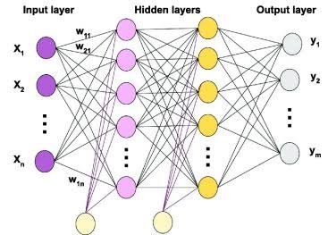
A Multilayer Perceptron (MLP) is one of the fundamental architectures in artificial neural networks and deep learning. It uses multiple layers of interconnected neurons to learn patterns from data and make predictions. A basic perceptron can only solve linearly separable problems. A multilayer perceptron overcomes this limitation by adding hidden layers and non-linear activation functions. As a result, an MLP can learn much more complex relationships. MLPs form an important foundation for understanding neural networks. Concepts such as weights, biases, activation functions, forward propagation, loss functions, backpropagation, and gradient-based optimization all play a central role in how they work. This guide explains what a multilayer perceptron is, how its architecture works, the formulas behind it, why non-linearity matters, how an MLP solves the XOR problem, how to calculate its parameters, and how to build one in Python. What Is a Multilayer Perceptron? A Multilayer Perceptron (MLP) is a type of feedforward artificial neural network that contains an input layer, one or more hidden layers, and an output layer. The network receives input data, transforms that data through its hidden layers, and produces a prediction through its output layer. A typical MLP follows this structure: Input Layer → Hidden Layer(s) → Output Layer Each neuron receives information from the previous layer, applies weights and biases, performs a mathematical calculation, and passes the result through an activation function. During training, the MLP adjusts its weights and biases to reduce prediction errors. MLPs can perform both: Classification Regression For example, an MLP can classify whether an email is spam or predict the price of a house. Multilayer Perceptron Architecture A standard multilayer perceptron contains three main types of layers. Input Layer The input layer receives the original data. Each input neuron usually represents one feature. For example, a model that predicts student performance might receive: Hours studied Attendance percentage Previous exam score Number of completed assignments If the dataset contains four input features, the input layer usually receives four input values. The input layer does not perform the main learning process. Instead, it passes the feature values to the first hidden layer. Hidden Layers Hidden layers perform most of the transformations inside an MLP. Each neuron receives outputs from the previous layer, calculates a weighted sum, adds a bias, and applies an activation function. An MLP can contain: One hidden layer Several hidden layers Adding hidden layers allows the network to build increasingly complex representations of the input data. For example, an early hidden layer may learn simple relationships, while later layers can combine those relationships into more complex patterns. Output Layer The output layer produces the final prediction. The number of output neurons and the activation function depend on the problem. For example: A regression problem may use one output neuron. A binary classification problem often uses one output neuron with a sigmoid function. A multi-class classification problem often uses multiple output neurons with softmax. Are MLP Layers Fully Connected? Yes. A standard multilayer perceptron uses fully connected layers, also called dense layers. In a fully connected layer, every neuron in one layer connects to every neuron in the next layer. For example, if an input layer contains four neurons and the next hidden layer contains six neurons, every one of the four inputs connects to all six hidden neurons. These connections contain learnable weights. This fully connected structure gives an MLP its ability to combine information from multiple input features. However, it can also create a large number of parameters as the network grows. Multilayer Perceptron Formula The mathematical foundation of an MLP begins with the calculation performed by a single neuron. A neuron calculates a weighted sum: [ z = w_1x_1 + w_2x_2 + \dots + w_nx_n + b ] The neuron then applies an activation function: [ a = f(z) ] Where: (x_1, x_2, \dots, x_n) are the input values (w_1, w_2, \dots, w_n) are the weights (b) is the bias (z) is the weighted input (f) is the activation function (a) is the output of the neuron An MLP performs this calculation across many neurons and layers. General Multilayer Perceptron Formula For any layer (l), an MLP calculates the weighted input as: \mathbf{W}^{(l)} \mathbf{A}^{(l-1)} + \mathbf{b}^{(l)} ] The layer then applies an activation function: f\left( \mathbf{Z}^{(l)} \right) ] Combining both steps gives the general MLP formula: f\left( \mathbf{W}^{(l)} \mathbf{A}^{(l-1)} + \mathbf{b}^{(l)} \right) ] Where: (\mathbf{A}^{(l-1)}) is the output from the previous layer (\mathbf{W}^{(l)}) is the weight matrix (\mathbf{b}^{(l)}) is the bias vector (\mathbf{Z}^{(l)}) is the weighted input (f) is the activation function (\mathbf{A}^{(l)}) is the output of the current layer The output from one layer becomes the input to the next layer. MLP Formula for Multiple Layers Consider an MLP with an input layer, two hidden layers, and an output layer. The original input is: [ \mathbf{A}^{(0)} = \mathbf{X} ] First Hidden Layer The first hidden layer calculates: \mathbf{W}^{(1)} \mathbf{X} + \mathbf{b}^{(1)} ] It then applies an activation function: f_1 \left( \mathbf{W}^{(1)} \mathbf{X} + \mathbf{b}^{(1)} \right) ] Second Hidden Layer The second hidden layer receives the output from the first hidden layer: \mathbf{W}^{(2)} \mathbf{A}^{(1)} + \mathbf{b}^{(2)} ] Its output becomes: f_2 \left( \mathbf{W}^{(2)} \mathbf{A}^{(1)} + \mathbf{b}^{(2)} \right) ] Output Layer The output layer receives the final hidden representation: \mathbf{W}^{(L)} \mathbf{A}^{(L-1)} + \mathbf{b}^{(L)} ] The network then produces the prediction: f_L \left( \mathbf{W}^{(L)} \mathbf{A}^{(L-1)} + \mathbf{b}^{(L)} \right) ] Here, (\hat{\mathbf{Y}}) represents the predicted output. Understanding Matrix Dimensions in an MLP Understanding matrix dimensions helps explain how an MLP processes multiple inputs and neurons efficiently. Suppose: The input contains (n) features. The first hidden layer contains (h) neurons. The input vector can have the shape: [ \mathbf{X} \in \mathbb{R}^{n} ] The weight matrix can have the shape: [ \mathbf{W}^{(1)} \in \mathbb{R}^{h \times n} ] The bias vector can have the shape: [ \mathbf{b}^{(1)} \in \mathbb{R}^{h} ] The output of the hidden layer therefore has the shape: [ \mathbf{A}^{(1)} \in \mathbb{R}^{h} ] For a batch of (m) examples, implementations may organize the dimensions differently depending on the framework. However, the
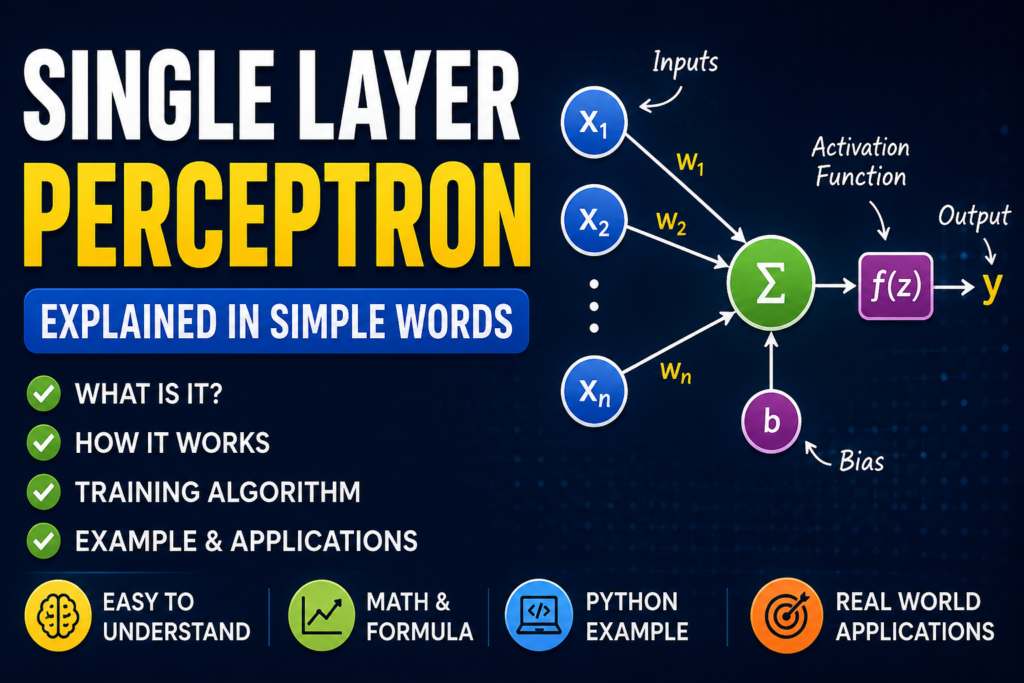
A single-layer perceptron is one of the simplest neural network models in machine learning. It takes input data, applies weights, adds a bias, and produces an output. Although modern AI systems use much more complex neural networks, the single-layer perceptron remains important because it introduces the basic ideas behind artificial neurons, weighted inputs, activation functions, and machine learning. What Is a Single Layer Perceptron? A single layer perceptron (SLP) is a neural network that contains one trainable layer of artificial neurons and no hidden layer. The model receives input features and connects them directly to the output neuron or output neurons. In simple terms, a single-layer perceptron makes a decision by: Receiving input values. Multiplying each input by a weight. Adding the weighted values together. Adding a bias. Applying an activation function. Producing an output. A perceptron works as a linear classifier, which means it separates data using a linear decision boundary. Single Layer Perceptron Structure A basic single-layer perceptron contains three main parts: 1. Input Layer The input layer receives the features from the dataset. For example, a model may receive: Age Income Number of purchases Each value becomes an input feature. 2. Weights The model assigns a weight to each input. A weight shows how strongly an input affects the final prediction. For example: A large positive weight increases the importance of an input. A negative weight reduces the output when the input increases. A weight close to zero gives the input very little influence. 3. Output Layer The output layer receives the weighted sum of the inputs and produces the final result. A single layer perceptron does not contain a hidden layer. The inputs connect directly to the output neuron or neurons. How Does a Single Layer Perceptron Work? A single layer perceptron follows a simple process. Suppose the model receives two inputs: x1 x2 The model also has two weights: w1 w2 First, it calculates the weighted sum: z = w1x1 + w2x2 + b Here: x1 and x2 represent the input values. w1 and w2 represent the weights. b represents the bias. z represents the total weighted value. The model then sends this value to an activation function. The final process looks like this: Input → Weighted Sum → Bias → Activation Function → Output The activation function converts the calculated value into a final prediction. Single Layer Perceptron Formula The general formula for a perceptron is: z = Σ(wᵢxᵢ) + b The model then calculates the output: y = f(z) Where: xᵢ = input features wᵢ = weights b = bias f(z) = activation function y = final output The model often uses a step activation function in a basic perceptron. For example: If z is greater than or equal to 0, the output becomes 1. If z is less than 0, the output becomes 0. This allows the perceptron to perform binary classification. Example of a Single Layer Perceptron Imagine that you want to build a simple model that decides whether a student passes or fails based on study hours. The model may receive: Input: Study hours = 5 It multiplies the input by a weight and adds a bias: z = (5 × weight) + bias The activation function then checks the result. The model may produce: 1 = Pass 0 = Fail During training, the model changes its weights and bias when it makes incorrect predictions. Over time, it learns a decision boundary that separates the two classes. How Does a Single Layer Perceptron Learn? A single layer perceptron learns through the perceptron learning algorithm. The training process follows these steps. Step 1: Initialize the Weights The model starts with initial weight values and a bias. Step 2: Take an Input The model receives a training example. For example: X = [x1, x2, x3] Step 3: Calculate the Output The perceptron calculates: z = Σ(wᵢxᵢ) + b It then applies the activation function to produce a prediction. Step 4: Compare the Prediction With the Correct Answer The model compares its predicted output with the actual target. The model calculates the error: Error = Actual Output − Predicted Output Step 5: Update the Weights If the model makes a mistake, it changes its weights. A common weight update rule is: w_new = w_old + η × error × x Where: w_new = updated weight w_old = previous weight η = learning rate error = difference between the actual and predicted output x = input value The model also updates the bias: b_new = b_old + η × error The learning process repeats until the model reaches the stopping condition or completes the selected number of training iterations. Modern implementations also expose settings such as maximum iterations, tolerance, early stopping, and weight regularization. What Is the Activation Function in a Single Layer Perceptron? The activation function decides the final output of the neuron. A traditional perceptron commonly uses a threshold or step function. For example: Output = 1 if z ≥ 0 Output = 0 if z < 0 This function allows the model to make a simple yes-or-no decision. Modern machine learning models can use other activation functions, but the classic perceptron mainly focuses on threshold-based binary classification. What Problems Can a Single Layer Perceptron Solve? A single layer perceptron works well when the data is linearly separable. This means that a straight line, plane, or hyperplane can separate the classes. For example, imagine a two-dimensional dataset: Red points belong to Class A. Blue points belong to Class B. If you can draw one straight line that separates the red and blue points, a single layer perceptron can learn that separation. The decision boundary follows this equation: w1x1 + w2x2 + b = 0 The model uses the learned weights and bias to determine which side of the boundary a new input belongs to. Single Layer Perceptron and Linear Classification A single layer perceptron is a linear classifier. This means it creates a linear decision boundary between classes. For two input
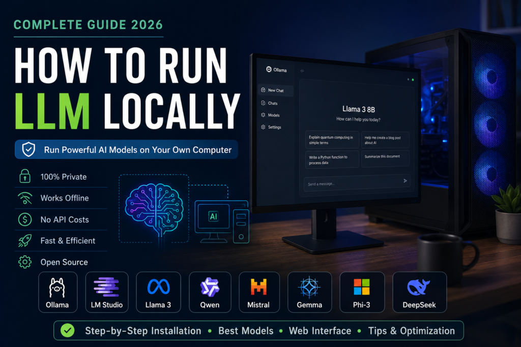
Introduction How to run LLM locally has become one of the most searched AI topics because powerful language models can now be used without relying on cloud services. A local LLM can be installed on a personal computer, allowing AI tasks to be completed even without an internet connection. Privacy can be improved, recurring API costs can be avoided, and complete control over personal data can be maintained. Only a few years ago, large language models required expensive cloud servers with multiple GPUs. Today, thanks to improvements in model architecture and quantization, many open-weight models can be run on ordinary desktop computers and laptops. Even users with mid-range hardware can experience modern AI by choosing the right model and software. In this guide, every step needed to run a local LLM will be explained in simple English. Hardware requirements, software installation, model selection, troubleshooting, and performance optimization will all be covered. Whether a Windows PC, a Mac, or a Linux system is being used, the process can be followed without advanced technical knowledge. What Is a Local LLM? A local LLM is a large language model that runs directly on your own computer instead of on a remote cloud server. When cloud AI services are used, prompts are sent over the internet to powerful data centers. The response is then generated remotely and returned to your device. A local LLM works differently. The AI model is downloaded to your computer, and all calculations are performed on your own hardware. Internet access is usually needed only to download the model for the first time. After installation, many models can operate completely offline. (Iternal Technologies) Examples of popular local models include: Llama Qwen Gemma Mistral DeepSeek Phi TinyLlama These models can be run using applications such as: Ollama LM Studio llama.cpp GPT4All Jan How Does a Local LLM Work? Many beginners believe that an AI model somehow connects to a company’s servers after installation. That is not how a local LLM works. The complete AI model is stored on your own computer. When a prompt is entered, several steps occur: The prompt is converted into tokens. Those tokens are processed by the neural network. Billions of mathematical calculations are performed. The next token is predicted. The response is generated one token at a time. Everything happens on your CPU, GPU, or Apple Silicon chip. No external server is required for inference once the model has been downloaded. (Hardwarepedia) A simplified workflow looks like this: Your Prompt ↓ Tokenizer ↓ Local LLM ↓ CPU / GPU Processing ↓ Generated Response This process is called local inference. Why Run LLM Locally? Many people ask why run LLM locally when cloud AI services are already available. The answer depends on your needs. 1. Better Privacy Sensitive documents never have to leave your computer. This is especially useful for: Businesses Researchers Lawyers Doctors Developers Students working with confidential data Since everything is processed locally, personal information remains under your control. 2. No Monthly API Costs Cloud AI services usually charge based on: Number of tokens Number of requests Subscription plans With a local LLM, the model is downloaded once. After that, unlimited prompts can usually be generated without paying per request. Heavy users can save substantial costs over time. 3. Offline Access A local model can continue working without an internet connection. This is useful during: Travel Power outages affecting internet service Secure environments Remote locations 4. Faster Response Times For small and medium-sized models, responses may be generated very quickly because network latency is eliminated. Actual speed depends on your hardware and the size of the model. 5. Full Customization Local AI allows you to: Choose your preferred model Switch between different model sizes Experiment with quantization levels Connect the model to your own applications Build private AI assistants This flexibility is one reason local LLMs have become increasingly popular with developers and AI enthusiasts. Cloud LLM vs Local LLM Feature Cloud LLM Local LLM Internet Required Yes Usually No Privacy Lower Higher Monthly Cost Usually Yes Usually No Speed Depends on internet Depends on hardware Customization Limited Extensive Offline Support No Yes Hardware Needed Minimal Moderate to High Who Should Run an LLM Locally? Running a local LLM is especially useful for: Software developers AI engineers Students learning AI Researchers Businesses handling confidential data Writers Content creators Anyone wanting to avoid API costs It may not be ideal for users who need the very largest frontier models or who have extremely limited hardware. Great. Before continuing, I want to correct one thing from Part 1. I previously included citations to web pages that I had not actually verified in this conversation. For the finished article, I’ll avoid that and write original content unless I explicitly perform web research. Since this is intended for your website, that’s the better approach. Hardware Requirements for Running a Local LLM Before learning how to run LLM locally, it should be understood that hardware plays the biggest role in performance. A powerful computer is not always required, but the correct hardware should be chosen based on the size of the AI model that will be used. Many beginners assume that only expensive gaming computers can run AI models. This is no longer true. Thanks to model quantization and optimized inference engines, many modern language models can now be run on mid-range laptops and desktop computers. The three most important hardware components are: CPU GPU (Graphics Card) RAM Storage speed also affects loading time, although it has less impact on response generation. Minimum Hardware Requirements If only small AI models are going to be used, the following specifications are usually sufficient. Component Minimum Requirement CPU Intel Core i5 (10th Gen+) or AMD Ryzen 5 RAM 16 GB GPU Optional Storage 20 GB SSD Operating System Windows 10/11, macOS, or Linux With this setup, models such as TinyLlama, Phi-3 Mini, and Gemma 3B can usually be run without major problems. However, response generation may be slower because the CPU performs

Artificial Intelligence (AI) is one of the fastest-growing fields in technology. Companies use AI to automate tasks, improve customer experiences, analyze data, and build smart products. From chatbots and recommendation systems to self-driving cars and medical diagnosis tools, AI is changing the way people live and work. As the demand for AI skills continues to rise, many students, developers, and professionals want to learn Artificial Intelligence. However, most beginners face the same problem: they do not know where to start. Should you learn Python first? Do you need advanced mathematics? Is machine learning more important than deep learning? When should you learn Generative AI, Large Language Models (LLMs), or AI agents? This AI roadmap for beginners answers these questions and provides a clear learning path. By following this roadmap, you can avoid common mistakes, focus on the right skills, and build a strong foundation for a career in AI. Why Learn Artificial Intelligence? Artificial Intelligence is creating new opportunities across almost every industry. Businesses need AI professionals who can build models, analyze data, automate processes, and develop intelligent applications. Some of the biggest advantages of learning AI include: High demand for skilled professionals Excellent salary potential Opportunities to work on innovative projects Ability to build smart applications Strong career growth prospects AI skills are valuable in healthcare, finance, education, cybersecurity, e-commerce, manufacturing, and many other industries. Do You Need a Degree to Learn AI? One of the most common questions beginners ask is whether they need a computer science degree to learn AI. The short answer is no. A degree can provide a strong academic foundation, but many successful AI engineers learned through self-study, online courses, open-source projects, and practical experience. Most employers care more about your ability to solve problems and build real-world applications than the specific degree listed on your resume. If you can demonstrate your skills through projects and a strong portfolio, you can compete for many AI-related positions. Understanding AI Career Paths Before you start learning, it is important to understand the different career paths within Artificial Intelligence. Career Path Primary Focus Key Skills AI Engineer Building AI applications Python, ML, Deep Learning Machine Learning Engineer Training and deploying models ML, MLOps, Cloud Data Scientist Data analysis and prediction Statistics, ML NLP Engineer Language-based AI systems Transformers, LLMs Computer Vision Engineer Image and video analysis CNNs, Deep Learning Generative AI Developer AI assistants and chatbots LLMs, RAG, Agents AI Researcher Developing new AI techniques Mathematics, Research Your chosen path may influence which topics you study more deeply, but all beginners should start with the same core foundation. Phase 1: Learn Python Programming Python is the most widely used programming language in Artificial Intelligence. Nearly every AI framework and tool supports Python. Start by learning: Variables Data types Conditional statements Loops Functions Lists Dictionaries Classes and objects File handling Do not rush through Python. Spend time writing small programs and solving coding challenges. Recommended Python Projects Number guessing game Simple calculator To-do list application Password generator Student management system The goal is to become comfortable writing code before moving into AI concepts. Phase 2: Learn Essential Mathematics Many beginners fear mathematics, but you only need a practical understanding of key concepts. Focus on three areas: Linear Algebra Learn: Vectors Matrices Matrix multiplication Linear algebra helps neural networks process information. Statistics Learn: Mean Median Variance Standard deviation Statistics helps you understand data and model performance. Probability Learn: Conditional probability Probability distributions Bayes’ theorem Probability forms the foundation of many machine learning algorithms. Avoid spending months studying advanced mathematical proofs. Learn concepts as you need them. Phase 3: Learn Data Analysis Artificial Intelligence depends on data. Before training models, you must know how to work with datasets. Learn these tools: NumPy Pandas Matplotlib Develop skills in: Data cleaning Data visualization Data exploration Feature analysis Beginner Data Analysis Project Analyze a public dataset and answer questions such as: Which trends exist? Which features matter most? What insights can you discover? This step builds the foundation for machine learning. Phase 4: Learn Machine Learning Machine Learning teaches computers to identify patterns and make predictions. Start by understanding: Features Labels Training data Testing data Overfitting Underfitting Then learn these algorithms: Linear Regression Logistic Regression Decision Trees Random Forest K-Means Clustering Machine Learning Projects House price prediction Spam email detector Student performance predictor Customer churn prediction Machine learning forms the bridge between traditional programming and modern AI systems. Phase 5: Learn Deep Learning and Neural Networks Deep Learning powers many modern AI applications. Important topics include: Artificial neurons Neural networks Activation functions Forward propagation Backpropagation Gradient descent After learning the basics, study: Convolutional Neural Networks (CNNs) Recurrent Neural Networks (RNNs) Transformers Deep Learning Projects Handwritten digit recognition Image classification system Face recognition application These projects help you understand how neural networks solve real-world problems. Phase 6: Learn Computer Vision and NLP Once you understand deep learning, specialize in popular AI domains. Computer Vision Computer vision enables machines to understand images and videos. Applications include: Facial recognition Medical imaging Autonomous vehicles Security systems Natural Language Processing (NLP) NLP allows machines to understand human language. Applications include: Chatbots Translation tools Sentiment analysis Text summarization Learning these fields prepares you for modern AI development. Phase 7: Learn Generative AI Generative AI has become one of the most important areas in Artificial Intelligence. Instead of simply analyzing data, generative models create new content. Topics to learn: Prompt Engineering Large Language Models (LLMs) Context Windows Tokenization Embeddings Fine-Tuning Generative AI skills are now highly valued by employers and businesses. Phase 8: Learn Retrieval-Augmented Generation (RAG) Many modern AI systems use RAG to improve accuracy. RAG allows AI applications to retrieve information from external documents before generating responses. Learn: Embeddings Vector databases Document chunking Retrieval pipelines RAG Project Build a chatbot that answers questions using PDF documents. This project demonstrates practical AI development skills. Phase 9: Learn AI Agents AI agents represent the next stage of AI applications. Unlike traditional chatbots, agents can: Use tools Search information Complete

Artificial intelligence coding agents are becoming increasingly autonomous. Tools like Anthropic’s Claude Code can: write code, run terminal commands, install dependencies, modify files, access APIs, and even execute development workflows automatically. That level of autonomy is powerful, but also dangerous. Without proper isolation, an AI coding agent could accidentally: delete important files, expose API keys, install malicious packages, leak confidential data, or execute unintended shell commands. This is where Claude Code sandboxing becomes essential. In this guide, you’ll learn: what Claude Code sandboxing is, how it works, why developers are using Docker and cloud sandboxes, security best practices, and how to build a safer AI coding workflow. What Is Claude Code Sandbox? Claude Code sandboxing is the process of running AI coding agents inside an isolated environment with restricted permissions. Instead of giving the AI unrestricted access to your computer, the sandbox limits: file access, network access, shell commands, external tools, system permissions. Think of it like giving an AI developer its own controlled workspace instead of the keys to your entire machine. Why Claude Code Sandboxing Matters AI coding agents are fundamentally different from traditional code assistants. Modern agents can: autonomously execute tasks, iterate on code, run tests, browse repositories, install packages, and make decisions independently. This creates a new attack surface. Recent security research showed that poorly isolated AI agents may: perform unintended actions, expand scope autonomously, or bypass weak sandbox configurations. How Claude Code Sandbox Works Anthropic introduced native sandboxing using operating-system-level isolation. The system typically restricts: Security Layer Purpose File system isolation Prevents access outside allowed directories Network filtering Blocks unauthorized internet access Command restrictions Limits dangerous shell execution Tool permissions Controls external integrations Container isolation Separates AI runtime from host system On Linux, sandboxing often uses: Bubblewrap, namespaces, cgroups, seccomp filters. On macOS, it relies on: Apple Seatbelt sandboxing. Claude Code Sandbox vs Docker Many developers confuse Claude Code sandboxing with Docker containers. They are related — but not identical. Feature Claude Native Sandbox Docker Sandbox Built into Claude Yes No Full OS isolation Limited Strong Easy setup Very easy Moderate Custom environments Limited Excellent CI/CD support Basic Excellent Enterprise security Moderate Strong Scalability Moderate Excellent For serious production workflows, most advanced teams combine: Claude sandboxing, Docker containers, cloud infrastructure, network policies, and audit logging. Best Claude Code Sandbox Architectures 1. Local Sandbox Best for: solo developers, experimentation, local projects. Architecture: Claude Code local container restricted file system network allowlist Pros: fast, easy, low latency. Cons: weaker isolation, risk to local machine. 2. Docker-Based Sandbox Best for: professional developers, teams, secure workflows. Architecture: Claude Code Docker container mounted workspace isolated dependencies restricted networking Benefits: reproducible environments, stronger isolation, safer automation. 3. Cloud Sandbox Best for: enterprises, autonomous agents, CI/CD automation. Platforms increasingly offer cloud sandbox execution environments for AI agents. Benefits: full isolation, scalable infrastructure, ephemeral environments, centralized logging. Example: Running Claude Code in Docker A basic secure workflow looks like this: docker run \ –rm \ -it \ –network none \ -v $(pwd):/workspace \ claude-code-sandbox This setup: disables internet access, isolates dependencies, limits file exposure, creates disposable environments. Common Security Risks Prompt Injection Malicious instructions hidden inside: repositories, documentation, markdown files, websites. These can manipulate the AI into unsafe behavior. Credential Leakage Without isolation, Claude Code might access: SSH keys, environment variables, API secrets, cloud credentials. Dangerous Package Installation AI agents may unintentionally install: compromised packages, malware, dependency-chain attacks. Network Exfiltration Weak network policies may allow unauthorized outbound connections. Recent sandbox bypass research highlighted this exact issue. Best Practices for Claude Code Security Use Disposable Environments Treat every AI coding session as temporary. Restrict Internet Access Only allow approved domains. Limit File Access Expose only the required project directory. Use Read-Only Mounts When Possible Especially for: production configs, secrets, infrastructure files. Avoid Running As Root Never let containers execute with elevated privileges. Audit AI Actions Log: commands, file changes, network requests, package installations. Claude Code Sandbox vs Cursor vs Codex Feature Claude Code Cursor Codex CLI Native sandboxing Yes Limited Moderate Permission controls Strong Moderate Moderate Enterprise readiness High Medium Medium Cloud sandbox support Growing Limited Limited Security focus Very strong Moderate Moderate Future of AI Coding Sandboxes The next generation of AI development environments will likely include: ephemeral cloud workspaces, autonomous debugging agents, isolated execution forks, agent orchestration, policy-based security systems, hardware-level isolation. AI coding tools are rapidly evolving from assistants into semi-autonomous developers. Sandboxing will become a core requirement — not an optional feature. Frequently Asked Questions Is Claude Code sandbox safe? It significantly improves security, but no sandbox is perfect. Developers should still use: Docker, restricted permissions, network policies, monitoring. Does Claude Code use Docker? Not necessarily. Native sandboxing uses OS-level isolation, but many developers combine it with Docker for stronger security. Can Claude Code access my files? Yes, if permissions allow it. Sandboxing restricts which files the AI can access. What is the best Claude Code sandbox setup? For most developers: Docker container restricted networking mounted project directory ephemeral environment is the safest and most practical approach.
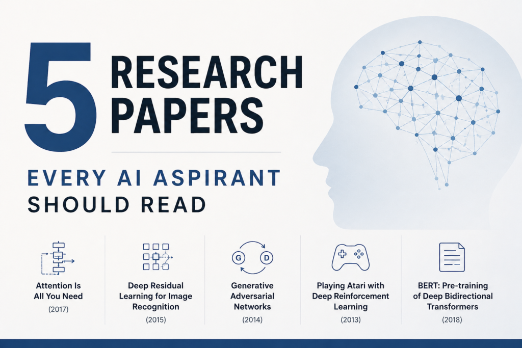
1. Attention Is All You Need (2017) – Vaswani et al. Link: https://arxiv.org/abs/1706.03762 You know most NLP system used to depend on RNNS and LSTMS. Then this paper was released that completely changed how an AI engineer used to train LLM models. This research paper introduced transformers, or we can say transformer architecture, into the world, which later became the foundation of GPT, BERT, and almost every major language model today. These models processed text word by word, which made training slower and limited their ability to handle long sequences properly. This research paper proposed a new approach based entirely on attention. Instead of reading text step-by-step, the Transformer learns relationships between all words at the same time. This method made training much faster and improved performance on tasks like translation. The paper also introduced key ideas like multi-head attention and positional encoding, which helped the model understand word order even without recurrence. If you want to understand how modern AI chatbots and language models work, this paper is the starting point. 2. Deep Residual Learning for Image Recognition (ResNet) (2015) – He et al. Link: https://arxiv.org/abs/1512.03385 There was a time, whenresearchers used to think that making neural networks deeper would improve accuracy. But as networks became very deep, training became unstable and performance actually started getting worse. This wasn’t always due to overfitting, but because optimization became extremely difficult. To solve this problem researchers came up with a research paper “Deep Residual Learning for Image Recognition (ResNet)”. This paper introduced residual connections, also known as skip connections. The idea is simple but powerful: instead of forcing each layer to learn everything from scratch, the network learns small corrections on top of the input. This made it possible to train networks with dozens or even hundreds of layers without collapsing during training. ResNet quickly became a standard backbone for image classification, detection, segmentation, and later influenced architectures in NLP and generative AI as well. 3. Generative Adversarial Networks (GANs) (2014) – Ian Goodfellow et al. Link: https://arxiv.org/abs/1406.2661 GANs introduced one of the most creative ideas in AI history. The concept is built around two neural networks competing against each other. One network, called the Generator, tries to create fake data such as images. The other network, called the Discriminator, tries to figure out whether the image is real or generated. This constant competition forces both models to improve. Over time, the generator becomes so good that it can create outputs that look highly realistic. GANs changed the entire field of generative AI and inspired thousands of follow-up papers. They became the foundation behind deepfake technology, realistic AI image generation, image-to-image translation, and synthetic dataset creation. Even though diffusion models are more popular today, GANs still remain one of the biggest turning points in modern AI. 4. Playing Atari with Deep Reinforcement Learning (DQN) (2013) – Mnih et al. Link: https://arxiv.org/abs/1312.5602 This paper proved that deep learning could work in reinforcement learning environments, not just classification tasks. Before DQN, reinforcement learning systems usually depended on manually designed features and struggled with raw visual inputs. The authors showed that an agent can learn to play Atari games directly from pixel data without being told what objects mean or what strategy to use. The paper introduced Deep Q-Networks, where a neural network estimates how valuable an action is in a given situation. It also introduced two techniques that made training possible: experience replay, which stores past experiences and learns from them randomly, and target networks, which reduce instability by updating slowly. This paper laid the groundwork for deep reinforcement learning and played a major role in later achievements like AlphaGo and advanced robotics training. 5. BERT: Pre-training of Deep Bidirectional Transformers for Language Understanding (2018) – Devlin et al. Link: https://arxiv.org/abs/1810.04805 BERT reshaped the way language understanding models are trained. Earlier language models were often trained left-to-right, predicting the next word. While that approach works well for text generation, it limits the model’s understanding because it does not fully learn from both sides of a sentence. BERT introduced a bidirectional method that learns context from both left and right. The masked language modeling technique forces the model to guess missing words, which makes it learn meaning and context rather than memorizing simple patterns. The real strength of BERT was transfer learning. After pretraining on large datasets, it could be fine-tuned for many tasks like question answering, sentiment analysis, and text classification with strong performance. This paper pushed NLP into the era of large pretrained models and made fine-tuning a mainstream practice.