sigmoid function

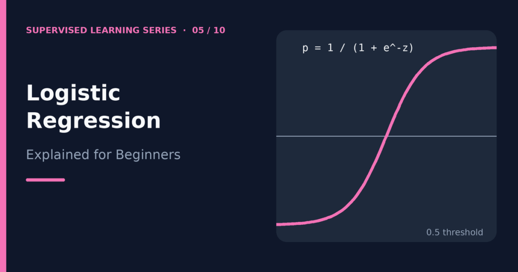
Logistic regression is a supervised learning algorithm that predicts the probability that an example belongs to a class, and then turns that probability into a class label. Despite its name, it is a classification method, not a regression method for predicting prices or temperatures. It answers questions such as “Is this email spam?” or “Will this customer cancel?” with a probability between 0 and 1. This guide explains logistic regression for beginners. You will learn how it uses the sigmoid function, what decision thresholds do, how to read coefficients, how the loss function works, and how regularization and multiclass problems fit in. A complete Python example follows. If you need a refresher on the task type, see Classification vs Regression in Machine Learning. Table of contents Why linear regression fails at classification The sigmoid function Probabilities and decision thresholds Reading the coefficients The loss function: log loss Multiclass classification Regularization Evaluation metrics Working Python example Strengths and limitations Frequently asked questions Conclusion Why linear regression fails at classification Imagine you code “passed” as 1 and “failed” as 0, then fit a straight line with linear regression. The line can output values like 1.4 or −0.3, which make no sense as probabilities. Outliers also tilt the line badly, so the predictions become unreliable near the boundary between the classes. Logistic regression solves the problem with a clever step. It keeps the familiar linear equation but passes its result through a function that squeezes any number into the range between 0 and 1. The squeezed number works as a probability. The sigmoid function The model first computes a weighted sum of the features, exactly as linear regression does. We call this value z: z = β₀ + β₁x₁ + β₂x₂ + … + βₚxₚ Then the sigmoid function (also called the logistic function) converts z into a probability p: p = 1 / (1 + e−z) In this formula, e is the mathematical constant 2.718…, and p is the predicted probability of the positive class. The curve has an S shape. Large positive values of z give a probability near 1. Large negative values give a probability near 0. A z of exactly 0 gives 0.5. z Sigmoid(z) = probability −4 0.018 −2 0.119 0 0.500 2 0.881 4 0.982 The sigmoid never reaches exactly 0 or 1. That behavior is useful, because the model always expresses at least a little uncertainty. Probabilities and decision thresholds A probability alone does not give you a class. You choose a decision threshold. The common default is 0.5: if p is at least 0.5, the model predicts the positive class, and otherwise it predicts the negative class. The default is not always the best choice. Suppose a model screens for a serious illness, and missing a sick patient is worse than ordering an extra test. You might lower the threshold to 0.3 so that the model flags more cases. You trade more false alarms for fewer misses. In the opposite situation, such as blocking a legitimate payment, you might raise the threshold. The threshold is a business or safety decision, not a property of the algorithm. Changing it does not retrain the model. It changes only how you convert probabilities into labels. The article on how to evaluate a supervised learning model shows how thresholds change precision and recall. Reading the coefficients Each coefficient β tells you how its feature moves z. A positive coefficient pushes the probability of the positive class up, and a negative coefficient pushes it down. A larger absolute value means a stronger push, provided that the features are on comparable scales. For a deeper reading, use odds. The odds of an event are p divided by (1 − p). For example, a probability of 0.8 equals odds of 4 to 1. Logistic regression is linear in the log-odds: log( p / (1 − p) ) = β₀ + β₁x₁ + … + βₚxₚ This means that raising x₁ by one unit adds β₁ to the log-odds, or multiplies the odds by eβ₁. If β₁ equals 0.7, the odds multiply by about 2.0 for each one-unit increase, with the other features held constant. Notice that the effect on the probability itself is not constant. It depends on where you start on the S-curve. As with linear regression, a coefficient describes an association in the data. It does not prove that the feature causes the outcome. The loss function: log loss Linear regression minimizes squared errors. Logistic regression uses a different loss, called log loss or binary cross-entropy, because squared error on sigmoid outputs creates a bumpy loss surface that is hard to optimize. For one example with true label y (0 or 1) and predicted probability p, the loss is: loss = −[ y × log(p) + (1 − y) × log(1 − p) ] This formula has an intuitive meaning. If the true label is 1, the loss is −log(p). A confident correct prediction (p near 1) gives a loss near 0. A confident wrong prediction (p near 0) gives a very large loss. The model therefore learns to be right, and it learns to avoid being confidently wrong. The training process averages this loss over all training examples and uses an optimizer, a relative of the gradient descent idea, to find the coefficients that minimize it. Multiclass classification Standard logistic regression handles two classes. Real problems often have more, such as three wine varieties or ten digits. Two main strategies extend the model: One-vs-rest (OvR). The method trains one binary model per class, each separating that class from all the others. For a new example, it picks the class whose model gives the highest probability. Multinomial (softmax) regression. The method learns all the classes together. A function called softmax converts one score per class into probabilities that add up to 1. Scikit-learn’s LogisticRegression handles multiclass targets automatically, and its default solver uses the multinomial approach. You do not need to write any extra code. Regularization When a model