early stopping

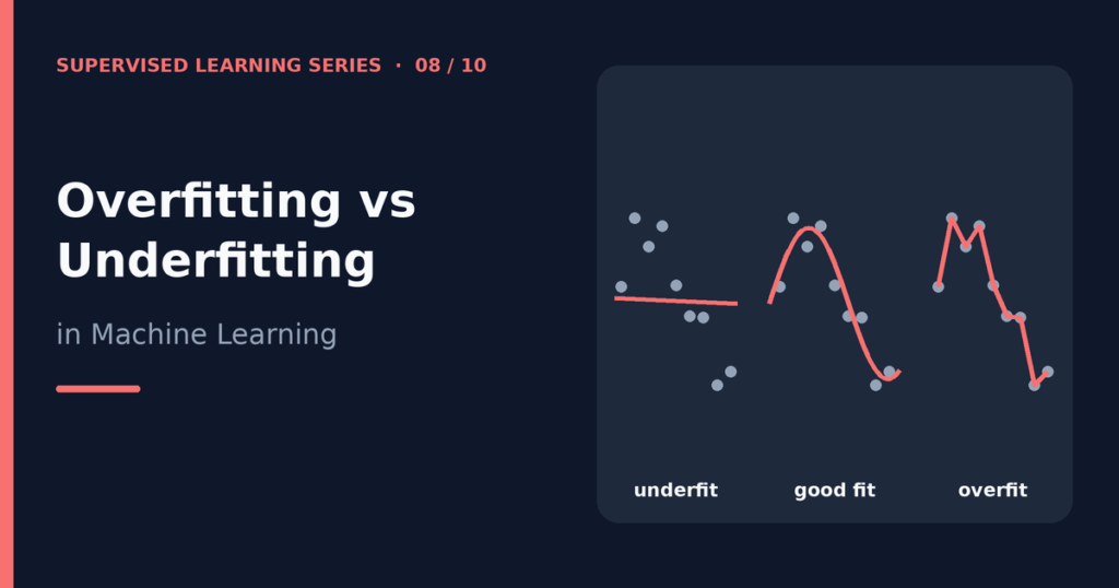
Overfitting vs underfitting describes the two most common ways a machine learning model fails to generalize. An overfit model learns the training data too closely, including its noise, so it scores well on training data but poorly on new data. An underfit model is too simple to capture the real pattern, so it scores poorly on both. A good model sits between the two. This guide explains both problems in plain language, shows how model complexity and the bias-variance trade-off connect them, and lists practical fixes: regularization, cross-validation, early stopping, better data, and feature selection. A Python experiment with real numbers makes the ideas concrete. Table of contents Generalization: the real goal What is overfitting? What is underfitting? How to tell them apart Model complexity The bias-variance trade-off How to reduce overfitting How to reduce underfitting Python experiment Frequently asked questions Conclusion Generalization: the real goal A supervised model trains on past examples, but you want it to work on future ones. We call this ability generalization. Overfitting and underfitting are the two ways generalization breaks down. If you are new to the training process, read What Is Supervised Learning? first. To measure generalization, you must test on data the model did not train on. That is why the series explains the split between training and test sets in Training Data vs Testing Data. Without that split, you cannot tell a model that learned from one that memorized. What is overfitting? Overfitting happens when a model fits the training data too well. It picks up random quirks and noise in the training set as if they were real patterns. A student who memorizes the answers to last year’s exam without understanding the subject behaves the same way. The student aces the old exam and fails a new one. Typical signs of overfitting: Very high training score, much lower validation or test score. Performance that varies a lot when you change the training sample slightly. A very flexible model, such as a deep unpruned decision tree or a network with many parameters trained for a long time. Common causes include a model that is too complex for the amount of data, too many features, noisy or mislabeled data, and training for too long. What is underfitting? Underfitting happens when a model is too simple to learn the real structure in the data. Fitting a straight line to data that follows a clear curve is a standard example. The model misses the pattern even on the training data. Typical signs of underfitting: Poor scores on both the training set and the test set. Training and test scores that are close together, but both disappointing. A model with strong restrictions, such as a very shallow tree, heavy regularization, or too few features. Common causes include a model with too little capacity, features that do not carry enough information, too much regularization, and training that stops too early. How to tell them apart Compare training performance with validation or test performance. The pattern tells you which problem you have. Situation Training score Validation or test score Diagnosis Both poor Low Low Underfitting (high bias) Large gap High Much lower Overfitting (high variance) Both good, small gap High Similarly high Good fit A learning curve gives a deeper view. You train the model on increasing amounts of data and plot the training and validation scores. If both curves stay low and close together, more data will not help, and you need a more capable model. If the training curve stays high and a big gap remains, more data or a simpler model can help. Model complexity Complexity describes how flexible a model is. Examples: A decision tree becomes more complex as max_depth grows. A polynomial model becomes more complex as its degree increases. A nearest-neighbor model becomes more complex as k gets smaller. A regularized model becomes less complex as its penalty grows stronger. As complexity rises, training error keeps falling, because a flexible model can bend to fit any training point. Validation error first falls and then rises again once the model starts fitting noise. The best complexity lies near the lowest point of the validation error curve. The experiment later in this article shows the pattern with a decision tree. The bias-variance trade-off Statisticians explain overfitting and underfitting with two kinds of error: Bias is error from wrong or overly simple assumptions. A high-bias model misses real patterns, and it underfits. Variance is error from sensitivity to the particular training sample. A high-variance model changes a lot when the training data changes, and it overfits. For squared-error problems, the expected prediction error splits into three parts: Expected error = bias² + variance + irreducible noise The irreducible noise comes from randomness in the data that no model can predict. You can reduce bias by using a more flexible model, but that tends to raise variance. You can reduce variance by simplifying the model, but that tends to raise bias. This tension is the bias-variance trade-off. Your goal is to find a balance that minimizes total error on new data, not to drive either term to zero. Ensembles show one smart way to ease the trade-off. A random forest averages many high-variance trees to cut variance without adding much bias. See Random Forest vs Decision Tree for details. How to reduce overfitting Collect more and better data More training examples make it harder for a model to memorize noise. Clean labels matter just as much, because a model will faithfully learn labeling mistakes. Simplify the model Reduce depth, remove layers, use fewer parameters, or choose a simpler algorithm. For trees, limits such as max_depth and min_samples_leaf, or cost-complexity pruning, control growth. The decision tree algorithm article covers these settings. Use regularization Regularization adds a penalty for complexity, usually for large coefficients. Ridge (L2) and lasso (L1) regularization do this for linear models. In logistic regression, the parameter C controls the strength, and smaller values mean stronger regularization. Neural networks use related tools such