
Radix Sort Algorithm: How It Works, Examples, and Python Implementation
A complete Radix Sort guide: traced LSD passes, counting sort internals, a correctness proof, Python and C++ code, base-256 variants, measured benchmarks, and complexity.
 Nov 21, 2026Published
42 min readReading time

Sorting is one of the most studied problems in computer science: take a collection of items and a rule that decides which item comes first, then rearrange everything until the rule holds everywhere.
Most classic algorithms solve it by comparing elements. Bubble sort compares neighbours and swaps them. Insertion sort compares a value with the sorted part on its left. Merge sort and quick sort split the list apart and compare values again while putting the pieces back together. Every one of them keeps asking the same question: “is this element smaller than that one?”
Radix Sort never asks that question. It does not compare whole numbers at all. Instead it looks at the individual digits of each number and groups the numbers by a single digit at a time, starting from the least significant digit on the right and moving left.
That one change has a real consequence. Comparison-based sorting cannot beat O(n log n) comparisons in the worst case, because every comparison only yields one bit of information. Radix Sort escapes that limit by making an assumption instead: the keys are integers (or short strings) whose digits can be inspected. In exchange, it can run in time that behaves like a linear function of n when the number of digits and the digit base are treated as constants.
This guide goes further than most tutorials on the subject. It works through the algorithm pass by pass, traces the counting sort subroutine cell by cell, proves why the least-significant-digit order is correct, gives you runnable Python for decimals, negatives, base 256, floats and strings, shows measured timings that challenge the usual “radix is always faster” claim, and covers the variants used in production systems.
Key takeaways
- Radix Sort is a non-comparison algorithm: it groups elements by digit instead of comparing them.
- LSD (least significant digit first) is iterative and stable; MSD (most significant first) is recursive and suits variable-length keys.
- Every digit pass must use a stable sort, normally counting sort, or earlier passes are destroyed.
- Time is O(d × (n + k)), space O(n + k) — linear in n only when d and k are fixed.
- Choosing the base is a real trade-off: more buckets means fewer passes but higher setup cost per pass.
- It suits bounded-width integers, IDs, dates and fixed-length codes — not arbitrary text or floating-point data without preprocessing.
On this page
- What is Radix Sort?
- A worked example, pass by pass
- Inside one pass: counting sort traced
- Why every pass must be stable
- Why LSD order is correct (proof)
- Algorithm and pseudocode
- Python implementation
- Negatives, signed ints and floats
- Choosing the radix (with benchmarks)
- Base-256 and bitwise radix sort
- MSD, in-place and hybrid variants
- Radix sort for strings
- Time and space complexity
- Performance reality check
- Advantages and disadvantages
- Radix sort vs other algorithms
- vs counting sort and bucket sort
- Applications
- Production optimisations
- Common mistakes
- Frequently asked questions
- Practice problems
What Is Radix Sort?
Radix Sort is a non-comparison sorting algorithm that orders integers by processing their digits one position at a time, using a stable sort for each digit.
“Non-comparison” means exactly what it says: the algorithm never checks whether one value is greater than or less than another value. It only computes digit values with division and modulo, and uses those digits as indexes into buckets. Because no pairwise comparison ever happens, the O(n log n) lower bound that applies to comparison sorting simply does not apply here.
Three terms make the rest of the algorithm easy to follow:
- Radix — the base of the number system in use, which is also the number of possible digit values. Base 10 gives ten possible digits (0–9), base 2 gives two, and base 256 gives 256. The radix decides how many buckets each pass needs.
- Digit position — the weight of a digit inside a number: ones (100), tens (101), hundreds (102), and so on.
- Pass — one complete sweep over the whole array that distributes the elements into buckets by the current digit and then collects them back into a single array.
Digit positions, weights, and the radix
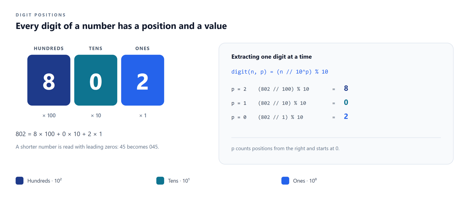
Every decimal number is a sum of digits multiplied by powers of ten. The number 802 is 8 × 100 + 0 × 10 + 2 × 1. Reading it from the right, the 2 sits in position 0, the 0 in position 1, and the 8 in position 2. To extract the digit at position p, divide by 10p and take the remainder modulo 10:
digit = (number // 10**p) % 10
This formula is the engine of the whole algorithm. It runs in constant time, needs no memory, and works the same way for a one-digit number, which simply behaves as if it had leading zeros.
LSD vs MSD Radix Sort
The digits can be processed in two directions, and the direction defines the variant.
LSD (least significant digit) Radix Sort starts at the rightmost digit and works towards the left. After the first pass the array is ordered by the ones digit, after the second pass by the last two digits, and after the final pass by the whole number. LSD is the version used in this article because it is simple, iterative, and naturally stable.
MSD (most significant digit) Radix Sort starts at the leftmost digit and then recursively sorts each bucket by the next digit inside it. It behaves like a generalised bucket sort and can stop early when a bucket holds a single element, which makes it attractive for variable-length strings and for keys that share long prefixes. The price is recursion, more bookkeeping, and a stability guarantee that is harder to maintain.
| Feature | LSD Radix Sort | MSD Radix Sort |
|---|---|---|
| Processing order | Right to left (ones, then tens, then hundreds) | Left to right (most significant digit first) |
| Structure | Iterative loop over digit positions | Recursive partitioning of each bucket |
| Stability | Stable, provided the digit sort is stable | Can be made stable with extra care |
| Best for | Fixed-width integers and fixed-length keys | Variable-length strings and shared prefixes |
| Early exit | No — every digit is always processed | Yes — a bucket with one item is finished |
| Memory | One output buffer of size n | Can be done in place, or with a full buffer |
| Passes | Always d | Between 1 and d in practice |
How Radix Sort differs from comparison-based sorting
Algorithms such as bubble sort and insertion sort learn about the data only through comparisons, so they need roughly n log n of them. Radix Sort learns about the data through arithmetic on the digits instead, and it keeps information in buckets rather than in comparisons. In practice that means three things:
- Its running time depends on how many digits the largest key has, not on how the keys are arranged.
- It needs a second array to hold the numbers while they are being redistributed.
- It only works on data that can be broken into digits — integers, fixed-length identifiers, or characters.
A short history
Radix sort is older than electronic computers. It descends from the tabulating machines Herman Hollerith built in the late 1880s, and punched-card sorters were using the technique commercially by the early 1920s: an operator fed a deck into a machine that dropped each card into one of thirteen pockets based on a single column, then moved the read head to the next column and repeated the process. The physical deck went through one pass per column, exactly as the algorithm does today.
The first memory-efficient computer implementation was written in 1954 at MIT by Harold H. Seward. Earlier attempts had been considered impractical because the bucket sizes were unknown in advance; Seward’s contribution was a preliminary counting scan that computes every bucket’s size and offset before any element moves — the same two-phase structure that modern merge sort-style implementations of counting sort still use. That scan is, in effect, counting sort, which is why the two algorithms are so closely related.
How Radix Sort Works: A Worked Example
Take this unsorted array of non-negative integers:
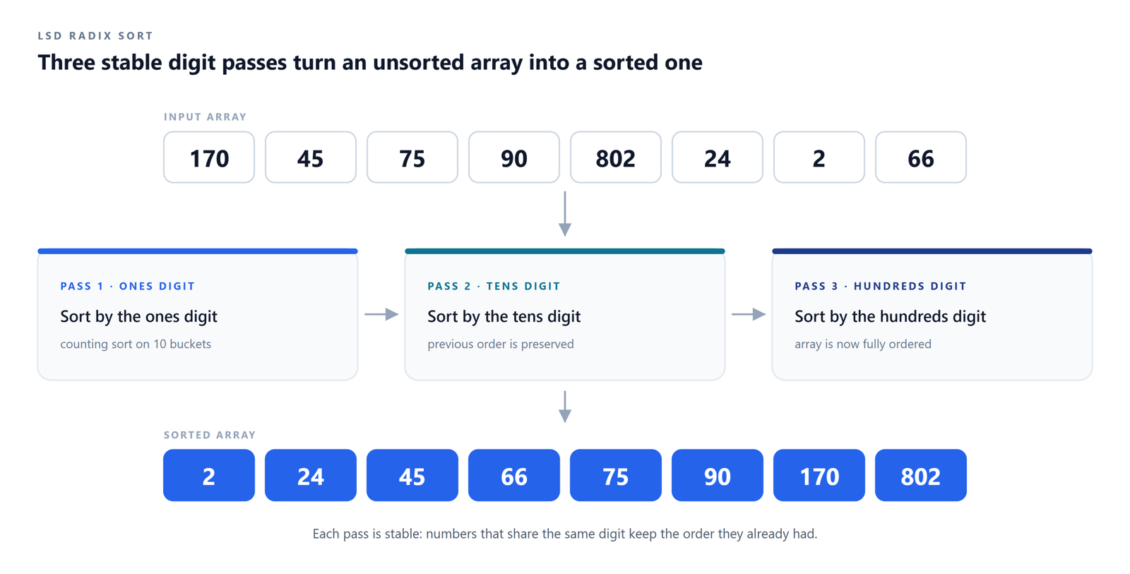
[170, 45, 75, 90, 802, 24, 2, 66]
The largest number, 802, has three digits, so the algorithm will make three passes. Because we work in base 10, each pass has ten buckets labelled 0 through 9. In every pass the numbers are dropped into the bucket that matches the digit currently being read, and then the buckets are collected from 0 to 9.
Pass 1: the ones digit
Read the last digit of every number: 170 → 0, 45 → 5, 75 → 5, 90 → 0, 802 → 2, 24 → 4, 2 → 2, 66 → 6. The buckets receive them in the order they appear:
- Bucket 0: 170, 90
- Bucket 2: 802, 2
- Bucket 4: 24
- Bucket 5: 45, 75
- Bucket 6: 66
- Buckets 1, 3, 7, 8, 9: empty
Collecting the buckets from 0 to 9 gives the array after the first pass:
[170, 90, 802, 2, 24, 45, 75, 66]
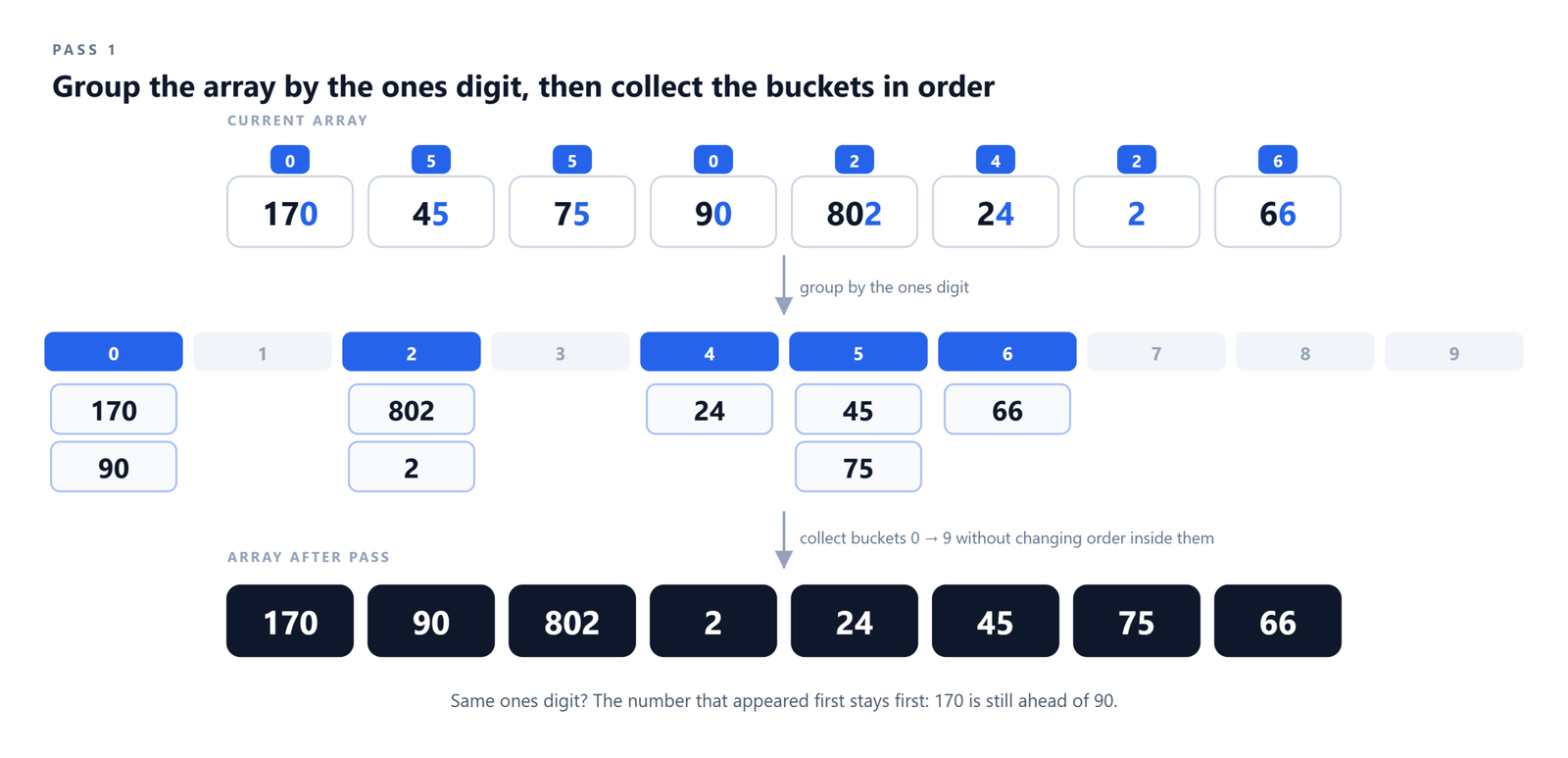
The array is now sorted by its last digit. That is a useful start, but it is not the answer yet.
Pass 2: the tens digit
Now read the second digit from the right: 170 → 7, 90 → 9, 802 → 0, 2 → 0, 24 → 2, 45 → 4, 75 → 7, 66 → 6. Note that 2 is treated as 02 — a missing digit counts as zero.
- Bucket 0: 802, 2
- Bucket 2: 24
- Bucket 4: 45
- Bucket 6: 66
- Bucket 7: 170, 75
- Bucket 9: 90
- Buckets 1, 3, 5, 8: empty
Collecting again from 0 to 9 gives:
[802, 2, 24, 45, 66, 170, 75, 90]
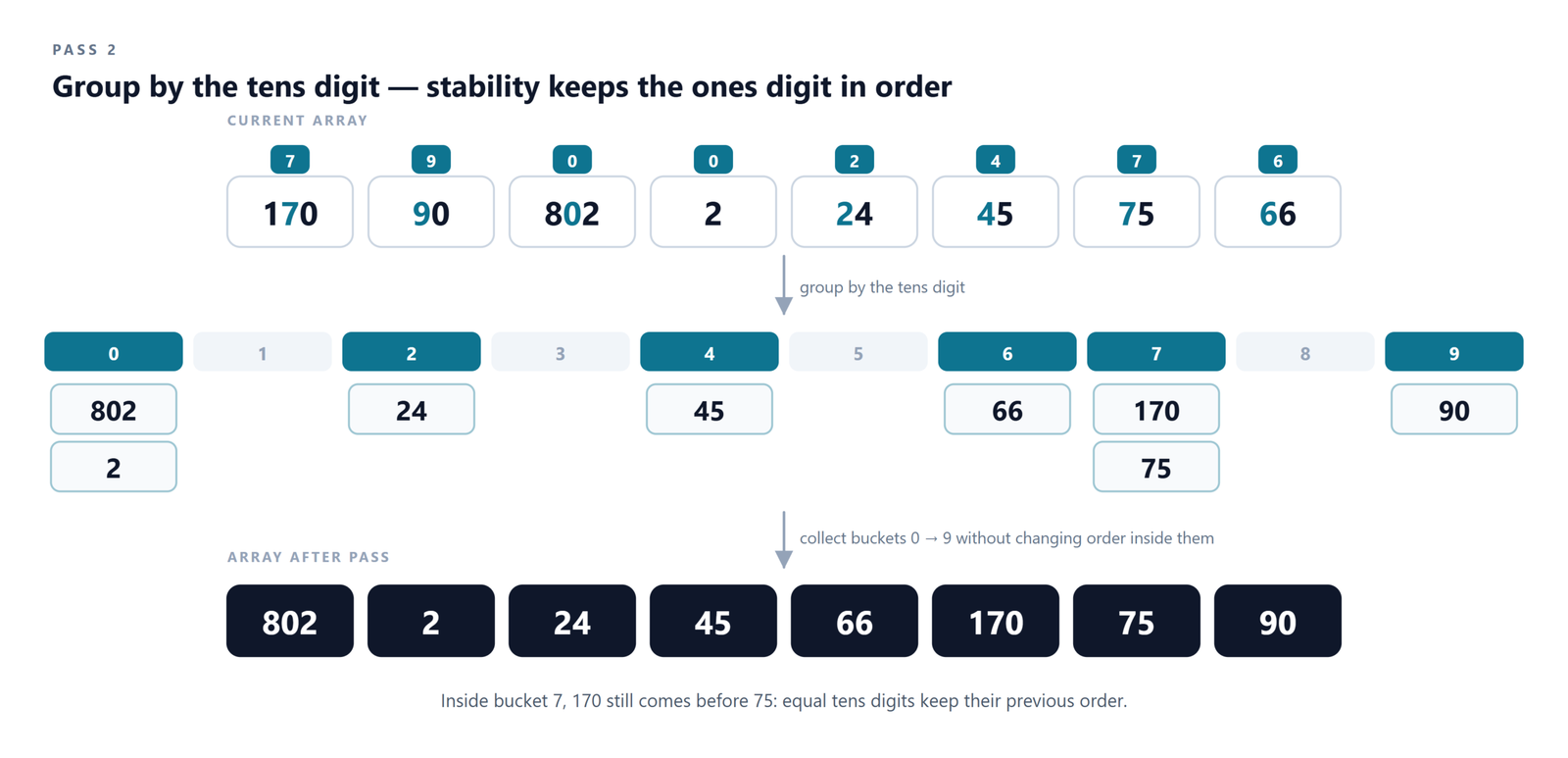
Something important just happened. Inside bucket 7, 170 comes before 75. Both arrived in that order from the previous pass, where they were ordered by their ones digits (0 and 5). The tens pass respected that earlier ordering instead of overwriting it.
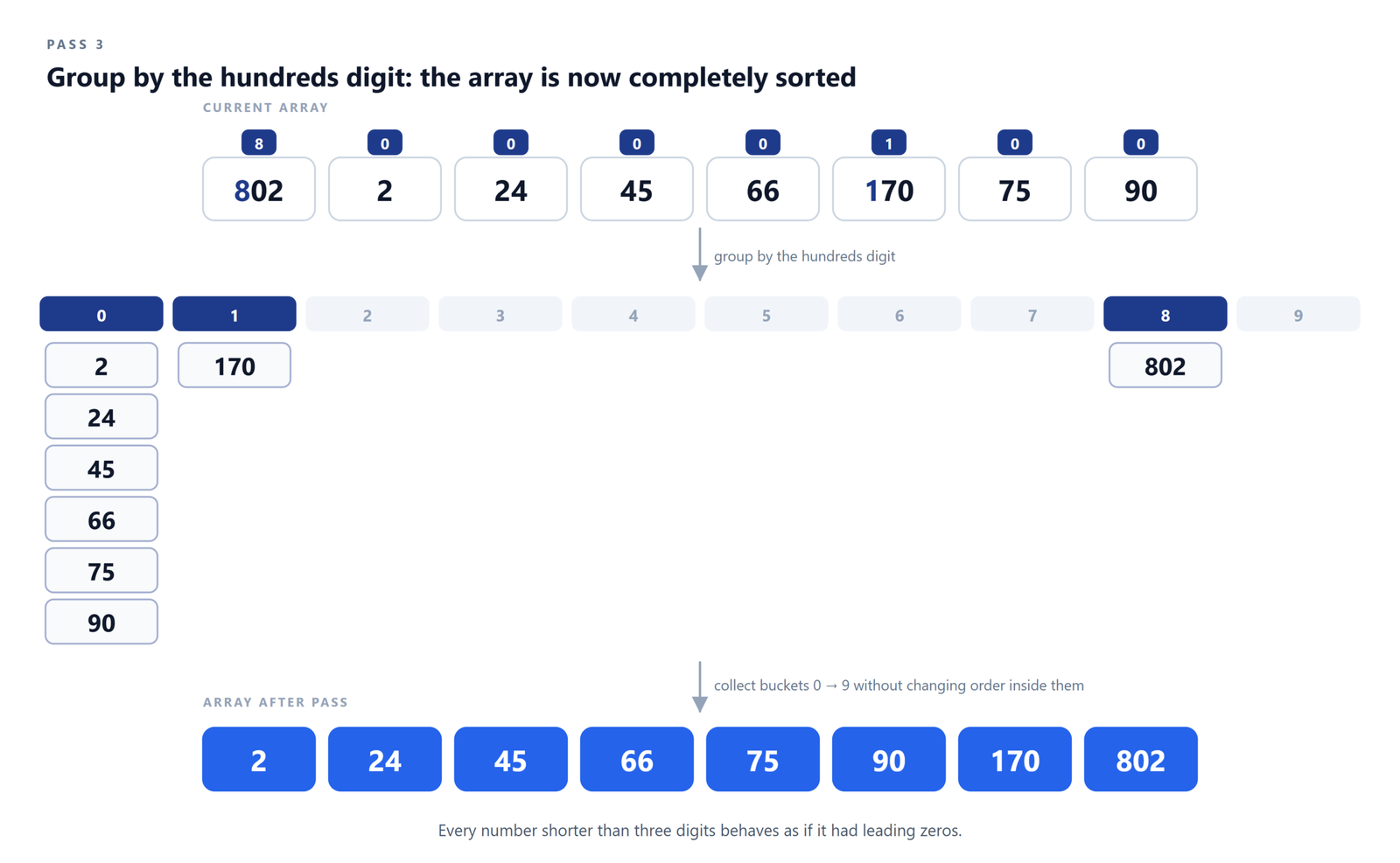
Pass 3: the hundreds digit
Finally read the third digit from the right: 802 → 8, 2 → 0, 24 → 0, 45 → 0, 66 → 0, 170 → 1, 75 → 0, 90 → 0.
- Bucket 0: 2, 24, 45, 66, 75, 90
- Bucket 1: 170
- Bucket 8: 802
- Buckets 2, 3, 4, 5, 6, 7, 9: empty
Collecting once more gives the final, fully sorted array:
[2, 24, 45, 66, 75, 90, 170, 802]
| Pass | Digit read | Array after the pass |
|---|---|---|
| Start | — | 170, 45, 75, 90, 802, 24, 2, 66 |
| 1 | Ones | 170, 90, 802, 2, 24, 45, 75, 66 |
| 2 | Tens | 802, 2, 24, 45, 66, 170, 75, 90 |
| 3 | Hundreds | 2, 24, 45, 66, 75, 90, 170, 802 |
Inside One Pass: Counting Sort, Traced
Every explanation of radix sort says “use counting sort on each digit”, and almost none of them show what counting sort does with the digit index. That gap is where most bugs are born, so here is pass 1 expanded into its actual cells.
The array is [170, 45, 75, 90, 802, 24, 2, 66] and the digit is the ones place. Reading left to right and incrementing a counter gives:
| Digit | 0 | 1 | 2 | 3 | 4 | 5 | 6 | 7 | 8 | 9 |
|---|---|---|---|---|---|---|---|---|---|---|
| Count | 2 | 0 | 2 | 0 | 1 | 2 | 1 | 0 | 0 | 0 |
| Running total | 2 | 2 | 4 | 4 | 5 | 7 | 8 | 8 | 8 | 8 |
The second row is the prefix sum. Each entry now holds the last slot that belongs to that digit. Digit 0 owns slots 0–1, digit 2 owns slots 2–3, digit 4 owns slot 4, digit 5 owns slots 5–6, and digit 6 owns slot 7.
Now walk the array backwards and place each element into the slot indicated by its counter, decreasing the counter afterwards:
| Step | Value | Digit | Slot used | Output array after placing |
|---|---|---|---|---|
| 1 | 66 | 6 | 7 | _, _, _, _, _, _, _, 66 |
| 2 | 2 | 2 | 3 | _, _, _, 2, _, _, _, 66 |
| 3 | 24 | 4 | 4 | _, _, _, 2, 24, _, _, 66 |
| 4 | 802 | 2 | 2 | _, _, 802, 2, 24, _, _, 66 |
| 5 | 90 | 0 | 1 | _, 90, 802, 2, 24, _, _, 66 |
| 6 | 75 | 5 | 6 | _, 90, 802, 2, 24, _, 75, 66 |
| 7 | 45 | 5 | 5 | _, 90, 802, 2, 24, 45, 75, 66 |
| 8 | 170 | 0 | 0 | 170, 90, 802, 2, 24, 45, 75, 66 |
The final row matches the array printed in the example, which is a useful sanity check. It also shows why the loop runs backwards. Walking from the end fills the highest remaining slot of each bucket first, so the element that appeared later in the input ends up later in the output. Reversing the loop direction would fill the lowest slot first and silently reverse every group of equal digits.
Two equivalent idioms. The backward loop above uses ending positions and decrements. The forward loop used in the Python code later in this article uses starting positions and increments. Both are stable; mixing one loop direction with the other’s offsets is the single most common way to break radix sort.
Why Every Pass Must Be Stable
A sorting algorithm is stable when elements that compare equal keep the order they already had. This detail is not a nicety in Radix Sort — it is the entire reason the algorithm works.
After pass 1 the array is ordered by the ones digit. When pass 2 sorts by the tens digit, the numbers whose tens digits are equal must remain ordered by their ones digit, because that ordering is the work pass 1 just finished. If the subroutine were unstable, numbers such as 170 and 75 could be swapped inside bucket 7 and the ones-digit ordering would be silently destroyed. Each pass would then wipe out part of the previous pass instead of building on it.
This is also why counting sort is the usual choice for each digit pass: it is stable, it runs in O(n + k) time, and it needs no comparisons. Merge sort is stable as well — but it costs O(n log n) per pass, which would remove the advantage of the digit approach entirely.
Worked counter-example. Suppose pass 2 used an unstable sort. Inside bucket 7 the two elements are 170 and 75, both with tens digit 7. An unstable sort might place 75 first. After pass 3, both land in bucket 0 along with 2, 24, 45, 66 and 90, and their relative order would be arbitrary — so the final array could read 75, 170 instead of 170, 75. The sort would return a wrong answer without ever raising an error. This is why testing only on already-sorted or distinct-digit inputs hides the bug.
Why LSD Order Is Correct
The claim to prove is: after pass p, the array is sorted by its lowest p+1 digits.
Base case. After pass 1 the array is sorted by the ones digit. That is exactly what pass 1 does, so the claim holds trivially.
Inductive step. Assume the array is sorted by its lowest p digits after pass p. Pass p+1 stably sorts by digit p+1. Take any two elements x and y with x appearing before y in the result. One of two things is true:
- Their digits at position p+1 differ, and x‘s is smaller — so x comes first in numeric order at that position.
- Their digits are equal, so stability guarantees x was already before y, and by the inductive hypothesis x is less than or equal to y on all lower digits.
Either way, x precedes y in the order defined by the lowest p+2 digits. That establishes the claim for p+1. After d passes every digit position has been considered, so the array is ordered by the complete key. ∎
The proof explains an asymmetry that puzzles many readers: it is the later passes that dominate. The most significant digit is processed last, so when it is processed every less significant digit has already been resolved and is preserved by stability. Processing the most significant digit first — the MSD variant — therefore needs recursion, because a single stable pass cannot preserve information it has not yet computed.
The Radix Sort Algorithm and Pseudocode
With the example understood, the algorithm itself is short. It is a loop over digit positions, wrapped around a stable digit sort.
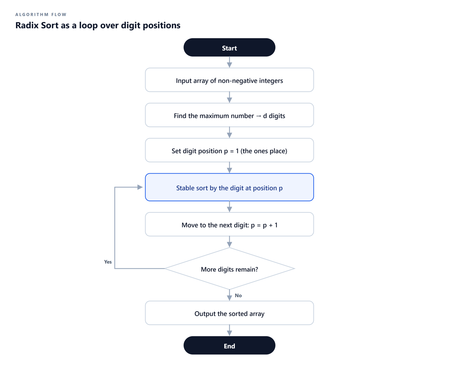
- Start.
- Input array of non-negative integers.
- Find the maximum number. Its digit count decides how many passes are needed.
- Set the digit position to the ones place (place = 1).
- Stable digit sort. Distribute the numbers into buckets by the digit at that position, then collect them back in bucket order.
- Move to the next digit by multiplying the place value by the base.
- Check whether digits remain. If the place value is still within the largest number, go back to step 5. Otherwise continue.
- Output the sorted array.
- End.
Expressed as language-independent pseudocode, with the digit sort spelled out:
RADIX_SORT(A, base)
    if A is empty
        return A
    M     ← maximum value in A
    place ← 1
    while M div place > 0
        COUNTING_SORT_BY_DIGIT(A, place, base)
        place ← place × base
    return A

COUNTING_SORT_BY_DIGIT(A, place, base)
    n      ← length(A)
    output ← new array of n slots
    count  ← new array of base zeros

    for i ← 0 to n - 1                      # 1. tally digits
        d ← (A[i] div place) mod base
        count[d] ← count[d] + 1

    total ← 0
    for d ← 0 to base - 1                   # 2. counts to start offsets
        c ← count[d]
        count[d] ← total
        total ← total + c

    for i ← 0 to n - 1                      # 3. place forward (stable)
        d ← (A[i] div place) mod base
        output[count[d]] ← A[i]
        count[d] ← count[d] + 1

    copy output back into A
This pseudocode uses start offsets with a forward placement loop, which is the mirror image of the backward loop traced earlier. Either pairing is correct; the two must not be mixed. Step 2 is what turns a histogram into bucket boundaries, and it is the step so many hand-written implementations get wrong.
Python Implementation of Radix Sort
The implementation below uses counting sort as the stable subroutine, needs no external libraries, handles an empty list, and returns the list sorted in ascending order.
def counting_sort_by_digit(values, place):
    """Stable sort by the digit at `place`."""
    n = len(values)
    output = [0] * n
    count = [0] * 10          # one counter per digit

    # 1. Count how often each digit appears
    for value in values:
        digit = (value // place) % 10
        count[digit] += 1

    # 2. Turn the counts into ending positions
    for digit in range(1, 10):
        count[digit] += count[digit - 1]

    # 3. Place from right to left to stay stable
    for i in range(n - 1, -1, -1):
        digit = (values[i] // place) % 10
        output[count[digit] - 1] = values[i]
        count[digit] -= 1

    # 4. Copy the result back
    for i in range(n):
        values[i] = output[i]


def radix_sort(values):
    """LSD Radix Sort for non-negative integers."""
    if not values:            # nothing to sort
        return values

    largest = max(values)     # number of passes
    place = 1                 # start at the ones place
    while largest // place > 0:
        counting_sort_by_digit(values, place)
        place *= 10           # move one digit left

    return values


arr = [170, 45, 75, 90, 802, 24, 2, 66]
radix_sort(arr)
print(arr)
How the code works, step by step
Finding the maximum number. largest = max(values) answers a single question: how many digits does the largest value have? That count is the number of passes. For 802 the answer is three, which is exactly what the worked example needed.
Walking the digit positions. The variable place starts at 1 and is multiplied by 10 after every pass. The loop condition largest // place > 0 becomes false once place has moved past the most significant digit, so the algorithm stops on its own — no digit count is computed separately.
Extracting a digit. Inside the subroutine, (value // place) % 10 isolates one digit. For 802 with place = 10 the computation is (802 // 10) % 10 = 80 % 10 = 0, which is the tens digit.
Counting sort as the stable subroutine. The counting sort runs in four moves. It counts how many numbers land in each of the ten buckets, converts those counts into ending positions with a running total, writes each number into its final slot, and copies the scratch array back. The result is a stable redistribution into digit order.
Preserving stability. The placement loop deliberately runs backwards, from the last element to the first. Because the ending position of each bucket shrinks after every insertion, walking backwards fills the rightmost slot of a bucket with the element that came last in the input, which keeps equal digits in their original relative order. Iterating forwards instead would reverse that order and break the algorithm.
Handling an empty array. if not values: return values returns immediately, so max() is never called on an empty sequence.
A base-agnostic version
Hard-coding 10 is convenient for teaching and wasteful in practice. The same code generalises to any base by replacing the modulus and the multiplier — and it is the version you want when the base becomes a tuning parameter.
def radix_sort_base(values, base=256):
    """LSD radix sort in any base. base=10 -> decimal digits."""
    if not values:
        return values

    largest = max(values)
    place = 1
    while largest // place > 0:
        n = len(values)
        output = [0] * n
        count = [0] * base

        for value in values:
            count[(value // place) % base] += 1
        for d in range(1, base):
            count[d] += count[d - 1]
        for i in range(n - 1, -1, -1):
            d = (values[i] // place) % base
            output[count[d] - 1] = values[i]
            count[d] -= 1

        values = output       # reuse the buffer as the new input
        place *= base

    return values


print(radix_sort_base([170, 45, 75, 90, 802, 24, 2, 66], 256))
print(radix_sort_base([170, 45, 75, 90, 802, 24, 2, 66], 10))
One subtlety: this version builds a new list each pass and rebinds values, so it returns a fresh list rather than mutating the caller’s. That is usually what you want. If you need in-place semantics, copy at the end or swap two pre-allocated buffers between passes, as the C++ version below does.
Negatives, Signed Integers and Floating-Point Numbers
How to handle negative integers
The version above assumes non-negative integers, because a negative digit has no natural bucket. The usual fix is to separate the signs, sort the absolute values, and then rebuild the list:
def radix_sort_with_negatives(values):
    """Sort integers that may be negative."""
    negatives = [-v for v in values if v < 0]
    non_negatives = [v for v in values if v >= 0]

    radix_sort(negatives)      # sorts absolute values
    radix_sort(non_negatives)

    # Negatives ascend by magnitude: reverse and negate
    negatives = [-v for v in reversed(negatives)]
    return negatives + non_negatives


print(radix_sort_with_negatives([-5, 3, -100, 0, 42, -1]))
The absolute values of the negative numbers are sorted in ascending order, which puts the largest magnitude first after reversal and negation. The approach is easy to reason about, but it allocates two extra lists and runs the algorithm twice.
The sign-bit trick for fixed-width integers
A cheaper method exploits two’s-complement representation. For a 32-bit integer, adding 231 maps the signed range [−231, 231 − 1] onto [0, 232 − 1] while preserving order — which is the same as flipping the most significant bit. Sort the shifted values as plain unsigned integers, then subtract the offset:
OFFSET = 1 << 31

def radix_sort_int32(values):
    """Sort 32-bit signed integers via sign-bit flip."""
    shifted = [v + OFFSET for v in values]
    radix_sort(shifted)                  # unsigned order
    return [v - OFFSET for v in shifted]


print(radix_sort_int32([7, -3, 0, -2147483648, 2147483647, -1]))
This is a single extra pass over the data with no partitioning, which is why it is the standard technique in systems code. In a fixed-width language the subtraction wraps modulo 232; Python’s integers are unbounded, so the plain subtraction is enough.
Sorting floating-point numbers
Floats are not decimals, but IEEE 754 was designed so that their bit patterns can be compared as integers after one transformation: if the sign bit is set, invert every bit; otherwise set the sign bit. The resulting unsigned integer preserves the total order of the floats — negatives first, then positive zero, then positives.
import struct

def float_to_key(x):
    bits = struct.unpack("<Q", struct.pack("<d", x))[0]
    return (~bits) & 0xFFFFFFFFFFFFFFFF if bits >> 63 else (bits | 0x8000000000000000)

def key_to_float(k):
    bits = (k & 0x7FFFFFFFFFFFFFFF) if k >> 63 else (~k) & 0xFFFFFFFFFFFFFFFF
    return struct.unpack("<d", struct.pack("<Q", bits))[0]

keys = [float_to_key(x) for x in [3.5, -2.25, 0.0, -0.0, 1e300, -1e-300]]
radix_sort(keys)
print([key_to_float(k) for k in keys])
This works because IEEE 754 stores the exponent above the mantissa, so lexicographic order on the bits matches numeric order for same-signed values. Two caveats: −0.0 and +0.0 are distinct in this ordering, and NaNs have no meaningful position — filter them out before sorting if your data can contain them.
Choosing the Radix: Cost, Buckets and Measured Data
Every tutorial tells you the base is 10. In production code it almost never is. The base is a free parameter, and it decides how the work splits between passes and buckets.
If the largest key is M, the number of passes in base b is
d = floor(log_b(M)) + 1
The total work is roughly d × (n + b). Making the base larger shrinks d but grows b. Differentiating that trade-off gives a rough optimum near b ≈ n, but there is a second constraint that usually wins: the counter array must fit in cache. With 256 counters of 8 bytes the table is 2 KB and stays in L1; with 65,536 counters it is 512 KB and every pass pays for touching it.
| Base | Digits per byte | Passes for 32-bit ints | Counter table | Typical use |
|---|---|---|---|---|
| 2 | 1 bit | 32 | 2 entries | Binary radix / bitwise sorting |
| 10 | — | 10 (for 32-bit) | 10 entries | Teaching, decimal identifiers |
| 16 | 4 bits | 8 | 16 entries | Fixed-point, some embedded code |
| 256 | 8 bits | 4 | 256 entries | The default choice in C/C++/Rust |
| 65,536 | 16 bits | 2 | 65,536 entries | Large arrays, generous memory |
What the numbers actually look like
The table below is measured, not estimated. Each figure is the best of three runs of the same pure-Python implementation on CPython 3.14.4 (Windows 11, x64) sorting n random integers drawn uniformly from 0 to 109.
| n | Base 10 (10 passes) | Base 256 (4 passes) | Base 65,536 (2 passes) |
|---|---|---|---|
| 100,000 | 284 ms | 135 ms | 103 ms |
| 1,000,000 | 4,282 ms | 1,751 ms | 1,001 ms |
| n | Base 10, per pass | Base 256, per pass | Base 65,536, per pass |
|---|---|---|---|
| 100,000 | 28.4 ms | 33.7 ms | 51.4 ms |
| 1,000,000 | 428 ms | 438 ms | 501 ms |
Two effects are visible, and they explain almost every radix sort performance question:
- Pass count dominates at scale. At one million elements, base 256 is 2.45× faster than base 10, and it performs 2.5× fewer passes. The per-pass cost is nearly identical (428 ms versus 438 ms), so the speedup is almost exactly the pass ratio.
- Bucket setup dominates at small sizes. At one hundred thousand elements, base 10 costs 28.4 ms per pass while base 65,536 costs 51.4 ms — nearly double, even though it does less useful work per element. Zeroing 65,536 counters costs more than the work saved.
That gives a practical rule: pick the largest power-of-two base whose counter table still fits comfortably in cache, and only go wider when n is large enough to amortise the setup. For 32-bit integers in a compiled language, 8 bits per pass is the sweet spot, which is exactly what most standard library and GPU implementations ship.
Base-256 and Bitwise Radix Sort
The version used in real systems extracts digits with shifts and masks instead of division and modulo. For a machine integer, that is not a micro-optimisation — integer division typically costs tens of cycles, while a shift costs one, and it happens on every element of every pass.
digit = (value >> shift) & 0xFF      # base 256, one byte
digit = (value // place) % 256      # equivalent, slower
With 8-bit digits, a 32-bit integer needs four passes and 256 buckets. A 64-bit integer needs eight. The trade-off is that hexadecimal and octal display formats become impossible to read directly, which is why teaching material sticks to base 10.
Here is the same algorithm in C++, written the way it would appear in production. Note that it keeps two buffers and swaps them between passes, so no copy-back pass is needed:
#include <vector>
#include <cstdint>
#include <cstddef>

void radixSort(std::vector<std::uint32_t>& a) {
    constexpr int BUCKETS = 256;
    std::vector<std::uint32_t> tmp(a.size());

    for (int shift = 0; shift < 32; shift += 8) {
        std::size_t count[BUCKETS] = {};

        for (std::uint32_t v : a)            // tally
            ++count[(v >> shift) & 0xFF];

        std::size_t offset = 0;
        for (int i = 0; i < BUCKETS; ++i) {  // counts to start offsets
            std::size_t c = count[i];
            count[i] = offset;
            offset += c;
        }

        for (std::uint32_t v : a)            // place forward, stable
            tmp[count[(v >> shift) & 0xFF]++] = v;

        a.swap(tmp);
    }
}
The forward loop is stable here because each bucket’s offset only ever increases, so equal bytes are written in their original relative order. This is the mirror image of the backward loop in the Python version, and it avoids the final copy at the cost of one buffer swap.
What “bitwise radix sort” means
Some articles describe a binary radix sort: one pass per bit, with two buckets, 32 passes for a 32-bit integer. It is the same algorithm with k = 2, and it is the version usually used to explain in-place MSD partitioning. It is rarely the fastest choice — 32 passes over the data beats the arithmetic advantage — but it is elegant, needs only a single counter pair, and is the basis of in-place variants.
MSD, In-Place and Hybrid Variants
MSD: recursive partitioning
MSD radix sort sorts by the most significant digit, then recursively sorts each bucket by the next digit, and stops as soon as a bucket contains one element. It is naturally implemented with recursion:
MSD_SORT(A, lo, hi, shift)
    if hi - lo <= 1 or shift < 0
        return
    count ← new array of 256 zeros
    for i ← lo to hi - 1
        count[(A[i] >> shift) & 0xFF] ← count[...] + 1
    compute bucket boundaries by prefix sum
    distribute A[lo..hi) into buckets   # in place, or via a buffer
    for each bucket
        MSD_SORT(A, bucket_lo, bucket_hi, shift - 8)
The advantage is early exit: if every key in a bucket has the same remaining digit, that bucket is finished, which can shrink the effective number of passes below d for clustered data. The disadvantage is that distribution into an array in place requires a cycle-following permutation, and that permutation is not stable.
In-place MSD: binary quicksort and American flag sort
Binary MSD radix sort partitions on one bit at a time and can be done with two pointers — swap the current element to the back if its bit is 1, advance if it is 0, and recurse on both halves. It is often called binary quicksort, and it needs O(log n) stack space rather than O(n) buffer space.
Generalising to more buckets gives American flag sort: count each bucket, compute boundaries, then use cycle-leading swaps to move every element into its bucket without allocating. It is in-place and fast, but not stable, which rules it out for LSD-style use and for multi-key records where the original order matters.
| Variant | Extra memory | Stable | Passes | Good for |
|---|---|---|---|---|
| LSD + counting sort | O(n + k) | Yes | Always d | Fixed-width integers, records |
| MSD + buffer | O(n + k) | Yes | 1 to d | Strings, prefix-heavy keys |
| Binary MSD (in place) | O(log n) stack | No | Up to bits | Tight memory, embedded |
| American flag (MSD, in place) | O(k) + stack | No | Up to d | Large alphabets, tight memory |
Why real implementations are hybrids
Radix sort has a high constant factor per element: a bucket index, an array write, a counter update, and (in interpreted languages) a function call. Below some threshold, that overhead exceeds the cost of a simple comparison sort.
The standard fix is to stop the recursion early and finish small buckets with insertion sort, which is stable, in place, and extremely fast on short arrays. Thresholds in the literature range from 16 to 64 elements. Every serious implementation — std::stable_sort internals in some libraries, GPU radix sorts, suffix-array builders — uses a cutoff of this kind.
Radix Sort for Strings
Radix sort is not limited to numbers. Any key that can be decomposed into a sequence of symbols with a defined ordering can be radix sorted, with each character acting as a digit in a larger base. English text has an alphabet of about 100 usable characters; DNA has four; a byte string has 256.
LSD for fixed-length strings
If every string has the same length — a fixed-width account code, a country plus region prefix, a hash digest — LSD works unchanged: one pass per character position, from the last character to the first, with counting sort over the alphabet. This is the simplest correct approach and it is stable.
MSD for variable-length strings
Variable-length keys need MSD, because a shorter string has no character at a position where longer strings do. The convention that resolves it is an end-of-string sentinel that sorts before every real character. With that sentinel, MSD radix sort produces true lexicographic order and can stop descending into buckets that become empty or singular.
Lexicographic is not numeric. Applying character-by-character sorting to numbers written as text gives 1, 10, 2, 3 rather than 1, 2, 3, 10, because the sentinel sorts before 0. This is correct lexicographic behaviour and a common source of confusion in file listings and version strings. Pad numeric strings to a fixed width if you need numeric order.
Three-way radix quicksort
For large alphabets, plain MSD radix sort creates hundreds of near-empty buckets and wastes time on each. Three-way radix quicksort (Sedgewick) combines the two ideas: partition on one character into “less than”, “equal to” and “greater than”, recurse on the less-than and greater-than partitions conventionally, and recurse on the equal partition at the next character position. It inherits radix sort’s speed on common prefixes and quicksort’s robustness on wide alphabets, and it is the algorithm behind several production string-sorting libraries.
String radix sorting is not academic. Suffix arrays — the data structure behind full-text search, genome alignment and Burrows–Wheeler compression — are commonly built with an MSD radix pass followed by a doubling algorithm, and the DC3 suffix-array construction relies on radix sorting internally.
Time and Space Complexity of Radix Sort
Three quantities describe the cost:
- n — the number of elements to sort.
- d — the number of digit positions, that is, the digit count of the largest key.
- k — the radix, meaning the number of possible digit values. For decimal numbers, k = 10; for byte-wise sorting, k = 256.
| Case | Time complexity | When it applies |
|---|---|---|
| Best | O(d × (n + k)) | Same as average — input order is irrelevant |
| Average | O(d × (n + k)) | Any input |
| Worst | O(d × (n + k)) | Any input, including adversarial |
| Space | O(n + k) | Output buffer plus counter table |
| Stable | Yes | When each digit pass is stable |
These bounds describe the standard LSD implementation built on a stable counting sort, and they hold regardless of how the input is arranged. Radix Sort has no favourable or unfavourable input pattern the way quick sort does, so best, average, and worst case are identical. That predictability is an underrated property: there is no adversarial input that turns radix sort quadratic.
Why d passes. Each pass places the array in order with respect to one more digit position, starting from the least significant. After d passes every position has been considered, so the array is ordered by the complete key. There is no way to skip a digit, because each one carries information the later passes rely on.
Why each pass costs O(n + k). A counting sort touches each element a constant number of times: once to count digits, once to place them, once to copy them back. That is O(n). It also walks the whole bucket table twice, which is O(k). Together the pass costs O(n + k), and d passes multiply it.
Why this is linear in n. In the expression O(d × (n + k)), the values d and k are fixed properties of the key type, not of the collection size. Sorting 32-bit integers in base 256 always takes four passes with 256 buckets no matter whether there are a thousand numbers or a hundred million. Treating d and k as constants leaves O(n). For decimal numbers that are not bounded in width, d grows with the logarithm of the largest value, and the cost becomes O(n log M) where M is the maximum key.
The constant factor nobody mentions. Knuth analyses each pass as two scans — one to count, one to permute — giving Θ(2d(n + k)). Because counts are always over the whole array and permuting does not change them, all digits can be counted in a single initial scan, reducing the total to Θ((d + 1)(n + k)). That single-pass counting trick is what modern GPU implementations use, and it is why an “O(dn)” radix sort in a paper can be noticeably faster than the textbook version.
Where the space goes. Each pass needs an output array of n elements and a count table of k counters, so the extra memory is O(n + k). This is the main structural difference from in-place algorithms: Radix Sort trades memory for the ability to skip comparisons. Note that k is not always small — choosing base 65,536 means 65,536 counters, which is 512 KB before you store a single element.
Performance Reality Check: Where Radix Sort Really Wins
Almost every article on this topic ends with “radix sort is O(n), so it beats O(n log n) algorithms”. That conclusion does not survive measurement, and the reason is worth understanding because it decides when to use the algorithm at all.
Here is the same test data sorted three ways: CPython’s built-in sorted() — which is Timsort, written in C — and the pure-Python radix implementation from this article, in base 256.
| n (values up to 109) | sorted() — Timsort in C |
Radix, base 256, pure Python | Ratio |
|---|---|---|---|
| 100,000 | 19.9 ms | 135 ms | 6.8× slower |
| 1,000,000 | 335 ms | 1,751 ms | 5.2× slower |
The asymptotic advantage is real, but it is buried under a constant factor of roughly 50× in favour of compiled code. Every element of every pass runs as interpreted bytecode: a list index, a division, a modulo, a counter increment, a second index, a decrement. Timsort does its comparisons in machine code and exploits runs that random data still contains.
That does not make radix sort useless. It tells you where to use it:
- Compiled languages. The same four-pass structure in C, C++, Rust, Go or Zig runs a few instructions per element per pass. There, radix sort routinely beats quicksort on integer arrays of a million elements or more, and several standard-library and game-engine implementations choose it for that reason.
- Expensive comparisons. When comparing two keys costs far more than extracting a digit — long strings, composite records, locale-aware collation — the comparison-based lower bound becomes the bottleneck and radix sort’s arithmetic looks free.
- GPUs and SIMD. Radix sort parallelises almost perfectly because counting and scattering are data-parallel operations with predictable memory access. GPU libraries ship radix sort as the default integer sort for exactly this reason.
- Very large n with small keys. The crossover point moves with n: at a hundred million integers, a handful of linear passes wins decisively.
What this means in Python. For ordinary Python code, use sorted() or list.sort() — they are C-level Timsort and will beat any hand-written radix sort at every size you are likely to test. If you need a fast integer sort in Python, use NumPy: its stable sort (kind="stable") uses radix sort for integer dtypes, so you get the algorithm’s asymptotics without the interpreter overhead. Implement radix sort yourself to learn it, or to port it to a compiled language.
Advantages and Disadvantages
Radix Sort is a genuinely useful tool, but it is a specialised one. Its strengths come directly from its assumptions, and so do its weaknesses.
Advantages
- Linear-time behaviour under suitable assumptions. When the digit count and the radix are bounded, radix sort runs in time proportional to the number of elements.
- No element-to-element comparisons. Every decision is made from a digit value, so the O(n log n) lower bound for comparison sorting never applies.
- Predictable cost. Unlike quicksort, the running time does not depend on the order of the input; there is no bad case to guard against and no need for randomisation.
- Excellent for fixed-width keys. Integers, machine words, dates stored as numbers, and fixed-length identifiers all have a known d, which keeps the number of passes small and constant.
- Easily parallelised. Counting and scattering are data-parallel, and MSD buckets can be dispatched to independent processors.
- Stable when built on a stable subroutine. Records that share a key keep their original order, which matters when sorting by several fields in sequence.
Disadvantages
- Extra memory is required. The O(n + k) scratch array and counter table rule out radix sort where memory is tight.
- Performance depends on digit count and radix. Long keys mean many passes, and a large radix means a large counter table and poor cache behaviour.
- It is not universally efficient. For a few hundred elements, the constant factors of many passes can lose to a well-tuned comparison sort such as merge sort or Timsort.
- It needs a stable subroutine. The LSD variant only works when each digit pass preserves the order of equal digits, which adds a requirement the algorithm cannot relax.
- Not every data type fits. Negative numbers, floating-point values, and variable-length strings need extra handling before the digits can be extracted at all.
- Bad for arbitrary-length decimal input. If keys are unbounded integers, d grows with the logarithm of the value, and the linear advantage evaporates.
Use it / don’t use it
| Situation | Verdict |
|---|---|
| Millions of 32- or 64-bit integers, compiled language | Use it — usually the fastest option |
| Fixed-width IDs, dates-as-integers, timestamps | Use it — constant pass count |
| Sorting by several keys in sequence (stable passes) | Use it — stability is free |
| GPU / SIMD batch sorting | Use it — designed for it |
| Long text, mixed-type or locale-sensitive keys | Avoid — use a comparison sort |
| Fewer than a few thousand elements | Avoid — setup cost dominates |
| Memory-constrained embedded targets | Avoid in-place variant only if stability is not needed |
| Unbounded big integers | Avoid — d grows with the value |
Radix Sort vs Other Sorting Algorithms
The table below compares standard implementations. Treat the complexity as a description of growth, not as a guarantee about which program finishes first on a given machine.
| Algorithm | Approach | Average time | Worst-case time | Extra space | Stable |
|---|---|---|---|---|---|
| Radix Sort (LSD, base k) | Non-comparison; one stable pass per digit | O(d × (n + k)) | O(d × (n + k)) | O(n + k) | Yes |
| Radix Sort (MSD) | Recursive partitioning by leading digit | O(d × (n + k)) | O(d × (n + k)) | O(n + k), or in place | Only with a buffer |
| Counting Sort | Non-comparison; counts occurrences of each key | O(n + k) | O(n + k) | O(n + k) | Yes |
| Bucket Sort | Distributes into buckets, sorts each bucket | O(n + k) | O(n²) | O(n + k) | Yes, if the inner sort is |
| Quick Sort | Divide and conquer with a pivot partition | O(n log n) | O(n²) | O(log n) call stack | No |
| Merge Sort | Divide and conquer, then merge sorted halves | O(n log n) | O(n log n) | O(n) | Yes |
| Heap Sort | Selection sort driven by a binary heap | O(n log n) | O(n log n) | O(1) | No |
| Timsort | Merge sort with run detection and insertion sort | O(n log n) | O(n log n) | O(n) | Yes |
The pattern is worth noticing. Counting sort is the fastest of the five but only when the range of keys is small, because k is the number of distinct values rather than the number of digits. Radix Sort is essentially counting sort applied one digit at a time, which keeps k small (ten for decimal) while still handling large keys. Merge sort and heap sort remain the safe general-purpose choices, and quicksort’s O(n²) worst case is avoided in practice by randomised or median-of-three pivots.
Radix Sort vs Counting Sort vs Bucket Sort
These three are often confused because all of them avoid comparisons and all of them use buckets. They differ in what the bucket index means.
| Counting sort | Bucket sort | Radix sort | |
|---|---|---|---|
| Bucket index is | The key itself | The key scaled into a range | One digit of the key |
| Time | O(n + k), k = key range | O(n + k) average, O(n²) worst | O(d(n + k)) |
| Space | O(n + k) | O(n + k) | O(n + k) |
| Stable | Yes | Yes, if the inner sort is | Yes, if each pass is |
| Breaks down when | Keys span a huge range | Keys are badly clustered | Keys have many digits |
| Typical use | Small integer range, counts, histograms | Uniformly distributed floats | Fixed-width integers and IDs |
The practical relationship is: counting sort is a special case of radix sort with a single pass, and radix sort is counting sort applied digit by digit so that k stays small. Bucket sort is the odd one out because it assumes a distribution rather than a representation — it performs well on uniform data and badly on clustered data, while radix sort does not care about the distribution at all.
Applications of Radix Sort
Radix Sort appears wherever keys are short, numeric, and plentiful:
- Large collections of integers. Fixed-size machine integers have a constant number of digits, so the number of passes is known before the data is even read.
- Fixed-length identification numbers. Student IDs, order numbers, account numbers and invoice references all share a fixed width, which makes digit extraction trivial.
- Postal codes and phone numbers. These are digit sequences with a fixed structure, so they can be sorted by digit without conversion.
- Timestamps and event logs. A 64-bit epoch timestamp is an integer; sorting millions of log lines by time is a classic radix sort job.
- Suffix arrays and full-text indexes. The DC3 / Kärkkäinen–Sanders–Burkhardt suffix-array construction radix sorts internally, and MSD radix passes are standard in Burrows–Wheeler compression pipelines.
- Genomic data. DNA has a four-letter alphabet, so base-4 radix sorting of k-mers is extremely efficient.
- GPU and SIMD sorting. Libraries such as CUB and Thrust use radix sort as the default for integer keys because counting and scattering vectorise cleanly.
- Database and external sorting. Distribution-based partitioning in sort-merge pipelines uses the same digit-bucketing idea to create balanced runs.
- Histograms and percentiles. The counting pass alone gives you a histogram, which is often the real goal of the computation.
- Network lookups. Prefix-tree and multi-bit trie structures used in routing tables are radix structures, built by the same digit-at-a-time decomposition.
Radix Sort is a poor fit when keys are long and varied (such as arbitrary English text), when the dataset is small enough that comparison sorting wins on constants, or when memory is the limiting resource.
Optimisations Used in Production
Textbook radix sort and shipping radix sort differ mainly in constant factors. These are the changes that matter:
- Swap buffers instead of copying. Allocate two arrays once and alternate them each pass. This removes the copy-back loop, which is a full extra pass over the data.
- Count all digits in one scan. Instead of counting per pass, tally every digit of every key in a single traversal, then build all bucket offsets at once. This turns 2d scans into d + 1.
- Use shifts and masks. For power-of-two bases,
(v >> shift) & maskreplaces division and modulo, which are among the slowest integer instructions. - Insertion-sort the small buckets. Stop recursing when a bucket holds fewer than about 32 elements and finish it with insertion sort.
- Skip constant digits. If every key shares the same digit at a position — very common with clustered IDs — that pass changes nothing and can be skipped entirely.
- Pre-allocate and reuse. In managed languages, allocating an output array per pass creates garbage-collection pressure that can dominate the sort.
- Parallelise the counting pass. Split the input across threads, count locally, then merge the histograms before scattering.
- Fuse passes on GPUs. Warp-level ballot instructions can perform several bits per pass, which is how GPU radix sorts reach billions of keys per second.
Common Mistakes and How to Spot Them
Almost every broken radix sort fails in one of these ways. Each has a distinct symptom.
| Mistake | Symptom | Fix |
|---|---|---|
| Unstable digit sort (e.g. selection sort per digit) | Output correct only when digits are distinct | Use counting sort, or merge sort per digit |
| Backward loop with start offsets, or forward loop with end offsets | Groups of equal digits come out reversed | Pair the loop direction with the offset type |
| Forgetting the modulo, using only division | IndexError or wrong buckets | (v // place) % base |
| Counting array not reset between passes | Later passes produce nonsense | Reinitialise count inside the pass |
Using >= instead of > in the prefix loop |
Off-by-one, last element lost | Start at index 1, add the previous entry |
Assuming place *= 10 for every base |
Wrong pass count for base 256 or 16 | Multiply by the actual base |
| Fixed-width integer overflow in C | Infinite loop on large keys | Guard the loop with a shift count, not multiplication |
| Sorting negatives without preprocessing | Negative values land in bucket 0..9 by digit, order lost | Sign-bit flip or split-and-negate |
| Testing only on distinct digits | Stability bugs stay hidden | Include values that share every digit position |
A one-line test that catches most of them: sort an array containing [11, 11, 11] plus a few distinct values, and verify the relative order of duplicate meaningfully distinct records. Identical integers cannot reveal instability — you need records that are equal on the sort key but different in payload.
Frequently Asked Questions
Is Radix Sort a comparison-based algorithm?
No. Radix Sort never compares two elements with each other. It computes digit values arithmetically and uses them as bucket indexes, which is exactly why it is described as a non-comparison sorting algorithm and why the O(n log n) lower bound does not apply to it.
Is Radix Sort faster than Quick Sort?
Sometimes, but not always. For large collections of bounded-width integers in a compiled language, Radix Sort’s O(d × (n + k)) running time usually beats quicksort’s O(n log n). For small inputs, long keys, interpreted languages, or memory-constrained environments, quicksort is usually the better choice. There is no single winner for every input.
Why does Radix Sort require a stable sorting algorithm?
Each pass sorts by one digit, and the passes before it have already established an order among the remaining digits. A stable subroutine preserves that earlier order for elements with the same current digit. Without stability, every new pass would scramble the work of the previous one and the final array would not be sorted.
What is the time complexity of Radix Sort?
O(d × (n + k)), where n is the number of elements, d is the number of digit positions, and k is the radix. Because d and k are fixed for a bounded key type, the complexity is often written as O(n) for practical purposes. For unbounded integer keys it becomes O(n log M).
Can Radix Sort sort negative numbers?
Not directly, because a negative digit has no natural bucket. Two standard fixes exist: split the array into negative and non-negative values, sort the absolute values of the negatives, then reverse and negate them; or flip the sign bit so signed values map onto unsigned ones in the same order. Both are shown in the implementation section above.
What is the difference between LSD and MSD Radix Sort?
LSD starts at the least significant digit and moves left, always processing every digit position; it is iterative and stable. MSD starts at the most significant digit and recursively sorts each bucket by the next digit, which suits variable-length strings and can finish early for buckets with a single element.
Is Radix Sort stable?
LSD Radix Sort is stable as long as the digit subroutine is stable, which counting sort is. MSD Radix Sort can be made stable, but it requires a full output buffer and more careful implementation because each bucket is sorted independently. In-place MSD variants such as binary quicksort and American flag sort are not stable.
What is the radix, and how do I choose it?
The radix is the base of the digit system, equal to the number of buckets per pass. Base 10 is the teaching choice, base 256 is the practical default for machine integers, and base 65,536 reduces passes further at the cost of a much larger counter table. Choose the largest power-of-two base whose counters still fit comfortably in cache.
Can Radix Sort sort strings?
Yes. Treat each character as a digit in an alphabet-sized base. Use LSD for fixed-length strings, where every key has the same number of positions. Use MSD for variable-length strings, with an end-of-string sentinel that sorts before every character. Note that this produces lexicographic order, so “10” sorts before “2”.
Is Radix Sort in-place?
The standard LSD version is not: it needs an output array of n elements plus a counter table. In-place variants exist — binary MSD radix sort and American flag sort — but they are not stable, which makes them unsuitable when equal keys must retain their original order.
Does Python’s sorted() use radix sort?
No. CPython uses Timsort, a hybrid merge sort written in C. A pure-Python radix sort is slower than sorted() at every size we measured, because the interpreter overhead per element per pass outweighs the asymptotic gain. NumPy is different: its stable sort uses radix sort for integer dtypes.
What is the difference between Radix Sort and Counting Sort?
Counting sort indexes buckets by the whole key, so it needs one counter per possible value and only works when that range is small. Radix sort applies counting sort once per digit, so each pass needs only as many counters as there are digit values, which makes it practical for keys spanning billions of values.
When should I not use Radix Sort?
Avoid it for small arrays, for long or variable-length text keys, for memory-constrained environments, and for unbounded integers where the digit count grows with the value. In those cases a comparison sort such as Timsort or merge sort is simpler and usually faster.
Practice Problems
These exercises build the parts of the algorithm that tutorials usually skip. They are ordered by difficulty, and none of them require a specific platform.
- Trace by hand. Run LSD radix sort on
[329, 457, 657, 839, 436, 720, 355]and write down the array after each pass. Verify against the algorithm before writing any code. - Add a base parameter. Modify the implementation to sort in base 4, then confirm the result matches
sorted()for random input. - Make it stable for records. Sort a list of dictionaries by a numeric field, keeping insertion order among equal keys. Then break stability deliberately and observe the difference.
- Implement MSD with a cutoff. Write an MSD radix sort for fixed-width byte strings that switches to insertion sort below 32 elements.
- Sort signed 64-bit integers in place. Combine the sign-bit flip with a two-buffer implementation and measure how much the flip costs.
- Sort floating-point values. Apply the IEEE 754 key transform, then verify that the output matches
sorted()for random values, including negative zero. - Benchmark the base. Measure your implementation at bases 2, 16, 256 and 65,536 for n = 104, 105 and 106. Plot time against base and find the crossover.
Conclusion
Radix Sort is built on a single, memorable idea: instead of comparing numbers, look at one digit at a time and let a stable bucket sort do the work. Starting from the least significant digit, each pass refines the ordering of the array, and after d passes the whole number is in order.
Stability is the hinge on which everything turns. Because elements with equal digits keep their previous order, the result of one pass is never undone by the next. That is why counting sort, which is stable and linear in the number of elements plus buckets, is the natural partner for each digit pass — and why an unstable subroutine silently produces wrong answers instead of failing loudly.
The performance story is more nuanced than the complexity table suggests. Radix sort really is O(d × (n + k)), and with fixed-width keys that is linear in n. But “linear” describes growth, not speed: the constant factor per element is much larger than a comparison, and in an interpreted language that constant dominates completely. Radix sort wins where the per-element work is cheap and the data is large — compiled languages, GPUs, fixed-width integer keys — and loses where comparisons are already fast and the keys are short.
The engineering details are what separate a working implementation from a fast one: choosing the base to balance pass count against counter-table size, swapping buffers instead of copying, extracting digits with shifts rather than division, flipping the sign bit for negatives, and finishing small buckets with insertion sort. Each of those is a constant-factor change, and together they are the difference between a textbook exercise and a production sort.
For the right data it is elegant and fast; for the wrong data, a comparison sort is the simpler answer. If you would like to compare it with the algorithms it competes against, read our guides to the bubble sort algorithm, insertion sort algorithm, merge sort, and quick sort. When you are ready to move from sorting to searching, the ternary search algorithm and the binary search tree are natural next steps.