
SARSA Algorithm Explained: On-Policy Reinforcement Learning
Learn the SARSA algorithm: the on-policy update rule, a worked numerical example, a complete Python GridWorld implementation, and how SARSA differs from Q-learning on cliff walking.
 Nov 20, 2026Published
26 min readReading time
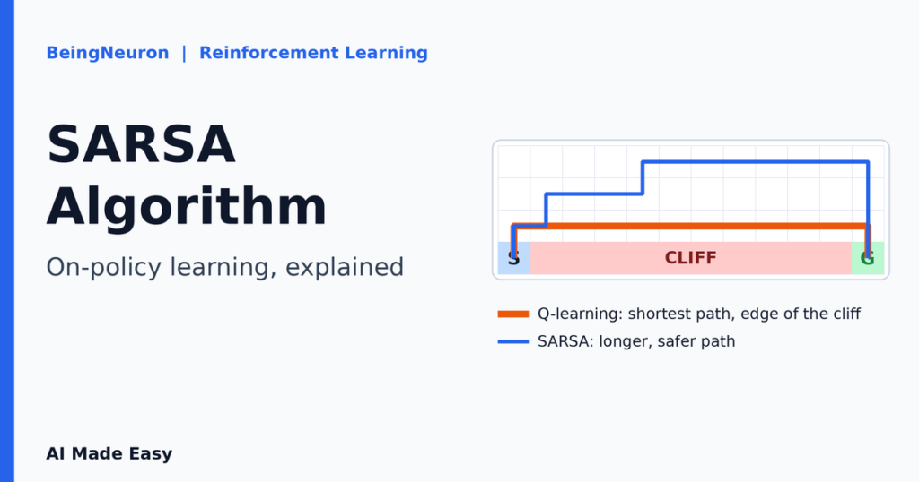
Picture a robot learning to walk to its charging dock along the edge of a cliff. Each time it explores, there is a small chance that a random step sends it over the edge. An agent that assumes it will always step perfectly will happily hug the edge, because the shortest route is optimal for a flawless walker. An agent that knows it sometimes stumbles will keep a safe distance. The SARSA algorithm is the learning method that builds this awareness of its own behavior into the numbers it learns.
SARSA is a close relative of Q-learning, and the two differ in a single term of one equation. That one term changes what the agent learns, how cautious it becomes, and what “on-policy” and “off-policy” mean in practice. In this guide you will see the update rule and every symbol in it, work through a numerical example that exposes the difference from Q-learning, follow the full algorithm, and build and run SARSA in Python with NumPy. A second experiment on the classic cliff-walking task shows the difference in measured results.
This article assumes you know the basics from What Is Reinforcement Learning? A Complete Guide and the Q-table idea from Q Learning Update Rule Explained: Formula, Algorithm & Python Example. We build directly on both and do not repeat their introductions.
What Is the SARSA Algorithm?
SARSA is a model-free, on-policy temporal difference algorithm that learns the value of each action in each state, using the actions its own policy actually takes. Like Q-learning, it stores an action value Q(s, a) for every state-action pair and improves it one step at a time, without needing a model of the environment. Unlike Q-learning, the value it learns belongs to the behavior the agent really follows, exploratory moves included.
The name is the recipe. Every update uses five items, in this order: State, Action, Reward, next State, next Action.
- State (s): where the agent is now.
- Action (a): the move the agent chooses in s.
- Reward (r): the number the environment returns for that move.
- Next state (s′): where the move leads.
- Next action (a′): the move the agent will choose in s′, selected by the same policy before the update is made.
The fifth item is what makes SARSA different. The agent must pick a′ before it can learn from the step it just took.
Why Was SARSA Developed?
SARSA grew out of temporal difference (TD) learning, the idea of improving a value estimate from the very next step instead of waiting for an episode to end. Rummery and Niranjan described the method in a 1994 Cambridge University technical report on online Q-learning with neural networks, where they called it “modified connectionist Q-learning”. The name SARSA came later and is credited to Richard Sutton. It is covered in Sutton and Barto’s textbook Reinforcement Learning: An Introduction.
The practical motivation is straightforward. In many real problems the agent learns while it acts, and its mistakes during learning have a cost. A method that evaluates the exact policy being followed, random exploration and all, gives value estimates that match how the agent really behaves. That makes SARSA a natural choice whenever the safety or quality of behavior during learning matters, not only at the end.
What Does On-Policy Learning Mean?
A policy, written π, is the rule that maps each state to the action (or action probabilities) the agent uses. Every learning algorithm involves two policies, and the difference between on-policy and off-policy methods is whether they are the same one.
- The behavior policy is the policy that actually picks actions and generates experience.
- The target policy is the policy whose value the algorithm is trying to estimate and improve.
In on-policy learning these are the same. SARSA acts with an epsilon-greedy policy and learns the value of that same epsilon-greedy policy. Its estimate Q(s, a) answers: “How much total reward can I expect if I take a now and then keep behaving the way I currently behave, random exploration included?”
Q-learning is off-policy. It also acts with an epsilon-greedy policy, but its update assumes the agent will act greedily afterwards, so it learns the value of the greedy policy instead. A fuller side-by-side comparison appears in the on-policy versus off-policy section below.
SARSA Update Rule Explained
The idea comes before the symbols. After each step, SARSA asks: “Was this move better or worse than I expected?” It builds a fresh estimate from what just happened, compares it with the old estimate, and nudges the old estimate toward the new one. The fresh estimate is the reward received plus the discounted value of the next state-action pair the agent is actually about to take.
| Symbol | Name | Meaning |
|---|---|---|
| Q(s, a) | Current action value | The agent’s present estimate of the return from taking a in s and then following its policy. It is both the value being replaced and part of the error term. |
| α | Learning rate | How far each update moves the old estimate toward the target (0 to 1). |
| r | Reward | The reward received after taking action a in state s. |
| γ | Discount factor | How much future reward counts compared with immediate reward (0 to 1). |
| s′ | Next state | The state the environment moved the agent into. |
| a′ | Next action | The action the current policy actually selects in s′. It will really be executed on the next step. |
| Q(s′, a′) | Value of the next pair | The current estimate for the state-action pair the agent is about to take, not the best one available. |
| r + γ · Q(s′, a′) | TD target | A fresh one-step estimate of Q(s, a). |
| target − Q(s, a) | TD error | The gap between the fresh estimate and the old one. Positive means “better than expected”. |
The theory behind it. The value of a policy π satisfies a self-consistency condition known as the Bellman expectation equation:
Qπ(s, a) = Eπ[ r + γ · Qπ(s′, a′) ]
Read it as: the true value of a pair equals the average, over what the environment and the policy do next, of the reward plus the discounted value of the next pair. SARSA cannot compute that average, so it samples it. Each real step supplies one sample of r, s′ and a′, and the update moves Q(s, a) a fraction α toward that sample. Because a′ comes from the policy, the quantity being estimated is Qπ for the agent’s own policy. Q-learning instead samples an equation for the best possible policy, which is why it has the max.
Terminal states. When s′ ends the episode there is no next action and no future reward, so the target is simply r. The code below treats this case explicitly.
Learning Rate, Discount Factor and Exploration in SARSA
Learning rate (α)
A large α overwrites old knowledge quickly, which speeds learning but makes estimates jumpy. A small α averages over many experiences, which is smoother but slower. Values between 0.1 and 0.5 are common for small tabular problems. If the environment is noisy, a smaller or gradually decreasing α usually works better.
Discount factor (γ)
With γ near 0 the agent is short-sighted and cares mostly about the next reward. With γ near 1, such as 0.9 or 0.99, it plans over a long horizon. A value that is too low can make a distant goal invisible; a value of exactly 1 is only safe in tasks that always end.
Exploration (ε)
Exploration plays a bigger role in SARSA than in Q-learning. In Q-learning, ε controls how the agent gathers experience, while the learned values describe the greedy policy. In SARSA, ε is part of the policy being evaluated, so it changes the learned values themselves. A larger ε makes SARSA more cautious around dangerous states, because it learns that random moves there are costly.
This gives SARSA a useful tuning dial, and a theoretical requirement. SARSA converges to the optimal policy when every state-action pair keeps being visited and the policy becomes greedy in the limit, usually by decaying ε toward zero over time (Singh et al., 2000). The standard step-size conditions on α also apply. In practice we approximate this with a decaying ε and a fixed, small α.
How Epsilon-Greedy Action Selection Works
Epsilon-greedy balances exploiting what the agent knows with exploring what it does not. At every decision the agent draws a random number. If it is below ε, the agent picks a uniformly random action. Otherwise it picks the action with the highest current Q-value.
Because the random choice can also land on the best action, the resulting policy has these probabilities, with |A| actions in total:
- The greedy action is chosen with probability 1 − ε + ε/|A|.
- Every other action is chosen with probability ε/|A|.
For example, with ε = 0.1 and four actions, the greedy action has probability 0.925 and each other action 0.025. These probabilities are exactly what the on-policy idea refers to: SARSA’s target uses an action drawn from this distribution. A common schedule starts ε near 1.0 so the agent explores widely, then shrinks it by a small factor each episode down to a floor such as 0.05.
SARSA Update: A Numerical Example
This example shows the difference from Q-learning with real arithmetic rather than words. The agent has just taken a move and now sits in state s′. Use these values:
- Current estimate: Q(s, a) = 5
- Learning rate: α = 0.5, and discount factor: γ = 0.9
- Reward just received: r = −1
- Values in the next state s′: up = 8.0, right = 2.0, left = 0.0, down = −9.0 (moving down leads into a pit)
The best action in s′ is “up”. But epsilon-greedy sometimes picks something else. The table shows what each algorithm computes depending on the action a′ that the policy actually selects.
| Next action a′ chosen | SARSA target | SARSA new Q(s, a) | Q-learning target | Q-learning new Q(s, a) |
|---|---|---|---|---|
| up (greedy, Q = 8.0) | −1 + 0.9 × 8.0 = 6.2 | 5 + 0.5 × (6.2 − 5) = 5.6 | −1 + 0.9 × 8.0 = 6.2 | 5.6 |
| right (explore, Q = 2.0) | −1 + 0.9 × 2.0 = 0.8 | 5 + 0.5 × (0.8 − 5) = 2.9 | −1 + 0.9 × 8.0 = 6.2 | 5.6 |
| down (explore, Q = −9.0) | −1 + 0.9 × (−9.0) = −9.1 | 5 + 0.5 × (−9.1 − 5) = −2.05 | −1 + 0.9 × 8.0 = 6.2 | 5.6 |
What the example shows. Q-learning produces 5.6 every time, whichever action is picked next, because it looks only at the maximum. SARSA’s result depends on the action the policy actually picked, so it ranges from 5.6 down to −2.05. A single SARSA update can look harsh, but notice what it represents: an exploratory step in that state really can end in a pit.
The average tells the real story. Suppose ε = 0.2. The greedy action “up” has probability 0.8 + 0.2/4 = 0.85, and each other action has probability 0.05. The expected next-action value is 0.85 × 8.0 + 0.05 × 2.0 + 0.05 × 0.0 + 0.05 × (−9.0) = 6.45. The expected SARSA target is therefore −1 + 0.9 × 6.45 = 4.805, compared with 6.2 for Q-learning. Over many visits, SARSA learns a lower value for stepping into this state, and that gap is the price of a risky neighbor that the agent will sometimes trip over. This is why SARSA learns routes that keep away from danger when exploring is costly.
SARSA Algorithm Step by Step
- Initialize. Create a Q-table with one row per state and one column per action, filled with zeros. Choose α, γ and an exploration schedule for ε.
- Start an episode. Place the agent in the starting state s.
- Choose the first action. Pick a from s using epsilon-greedy.
- Act. Take a, then observe the reward r and the next state s′.
- Choose the next action. Pick a′ from s′ using the same epsilon-greedy policy. This happens before the update.
- Update. Apply Q(s, a) ← Q(s, a) + α [ r + γ Q(s′, a′) − Q(s, a) ]. If s′ is terminal, the target is just r.
- Advance. Set s ← s′ and a ← a′. The action used in the update is the one executed next.
- Check for the end. If s′ was terminal, finish the episode. Otherwise return to step 4.
- Repeat. Lower ε a little and begin a new episode until training is done.
SARSA pseudocode
initialize Q[s][a] = 0 for every state s and action a
set alpha, gamma, epsilon, epsilon_min, epsilon_decay

for each episode:
    s = start_state
    a = epsilon_greedy(Q, s, epsilon)                 # choose the first action
    while s is not terminal:
        s_next, r = environment.step(s, a)
        a_next = epsilon_greedy(Q, s_next, epsilon)   # choose the NEXT action now

        if s_next is terminal:
            target = r
        else:
            target = r + gamma * Q[s_next][a_next]    # uses a_next, not the max

        Q[s][a] = Q[s][a] + alpha * (target - Q[s][a])
        s, a = s_next, a_next                         # a_next is the action taken next

    epsilon = max(epsilon_min, epsilon * epsilon_decay)
The most common SARSA bug is choosing a fresh action at the top of every step instead of carrying a′ forward. If you pick one action for the update and a different one to execute, the algorithm is no longer on-policy, because the value being learned would not match the action taken. The pseudocode avoids this by assigning a = a_next at the end of each step.
The GridWorld Environment
To keep the comparison fair, we reuse the same 4 × 4 GridWorld as the Q-learning article. The agent starts in the bottom-left cell (3,0) and must reach the goal in the top-right cell (0,3). Cells are written as (row, column), with row 0 at the top.
- Actions: up, down, left, right. Moving off the grid leaves the agent in place.
- Rewards: −1 for every ordinary move, +10 for reaching the goal, −10 for stepping into a pit.
- Pits: (1,1), (1,3) and (3,2). The goal and the pits end the episode.
- Best possible return: the shortest safe route takes 6 moves, so 5 × (−1) + 10 = +5.
SARSA Python Implementation with NumPy
The implementation below uses only NumPy. Install it with pip install numpy. Copy the stages in order into one file named sarsa_gridworld.py. I ran this complete script with Python 3.12.3 and NumPy 2.5.4, and the output shown below is from that run. Exact numbers can differ slightly on other NumPy versions, because random number streams are not guaranteed to be identical between releases.
Stage 1: Imports and environment
import numpy as np

SEED = 42  # makes every run reproducible

# Row 0 is the top row. Cells are written as (row, column).
N_ROWS, N_COLS = 4, 4
START = (3, 0)
GOAL = (0, 3)
PITS = {(1, 1), (1, 3), (3, 2)}

STEP_REWARD = -1.0
GOAL_REWARD = 10.0
PIT_REWARD = -10.0

ACTIONS = ["up", "down", "left", "right"]
ARROWS = ["↑", "↓", "←", "→"]
MOVES = [(-1, 0), (1, 0), (0, -1), (0, 1)]   # (row change, column change)

N_STATES = N_ROWS * N_COLS
N_ACTIONS = len(ACTIONS)


def to_state(cell):
    row, col = cell
    return row * N_COLS + col


def to_cell(state):
    return divmod(state, N_COLS)


def step(state, action):
    """The environment: apply an action, return (next_state, reward, done)."""
    row, col = to_cell(state)
    d_row, d_col = MOVES[action]
    new_row, new_col = row + d_row, col + d_col
    if not (0 <= new_row < N_ROWS and 0 <= new_col < N_COLS):
        new_row, new_col = row, col          # off the grid: stay in place
    next_cell = (new_row, new_col)
    if next_cell == GOAL:
        return to_state(next_cell), GOAL_REWARD, True
    if next_cell in PITS:
        return to_state(next_cell), PIT_REWARD, True
    return to_state(next_cell), STEP_REWARD, False
NumPy supplies the Q-table and the random number generator. The constants define the world: its size, the start, goal and pits, and the rewards. to_state flattens (row, column) into a single row number so the Q-table can be indexed by an integer. step is the environment. It takes a state and an action and returns the next state, the reward and a done flag that is True when the episode has ended at the goal or in a pit.
Stage 2: The Q-table and epsilon-greedy selection
def create_q_table():
    return np.zeros((N_STATES, N_ACTIONS))


def choose_action(q_table, state, epsilon, rng):
    if rng.random() < epsilon:
        return int(rng.integers(N_ACTIONS))                # explore: random action
    best_actions = np.flatnonzero(q_table[state] == q_table[state].max())
    return int(rng.choice(best_actions))                   # exploit: best action, ties broken randomly
The Q-table has one row per state and one column per action, all zeros, so the agent starts knowing nothing. choose_action implements epsilon-greedy exactly as described earlier. With probability epsilon it returns a random action. Otherwise it finds the action or actions with the highest Q-value. Ties are common early in training, when every value is 0, so the function chooses randomly among them rather than always picking “up”.
Stage 3: The SARSA update rule
def sarsa_update(q_table, state, action, reward, next_state, next_action,
                 done, alpha, gamma):
    current_q = q_table[state, action]
    if done:
        target = reward                                    # terminal: no future reward
    else:
        target = reward + gamma * q_table[next_state, next_action]
    td_error = target - current_q
    q_table[state, action] = current_q + alpha * td_error
    return td_error
This function is the formula line by line. current_q is Q(s, a). The target is r + γ · Q(s′, a′), and the code reads the value at next_action, the action the policy actually chose. A Q-learning version would replace that single lookup with np.max(q_table[next_state]). When done is true the target is just the reward. The TD error is the target minus the current value, and the last line adds α times that error.
Stage 4: Training loop
def train(episodes=500, alpha=0.1, gamma=0.9,
          epsilon_start=1.0, epsilon_min=0.05, epsilon_decay=0.99,
          max_steps=100, seed=SEED):
    rng = np.random.default_rng(seed)
    q_table = create_q_table()
    epsilon = epsilon_start
    episode_returns = []

    for _ in range(episodes):
        state = to_state(START)
        action = choose_action(q_table, state, epsilon, rng)    # first action
        total_reward = 0.0

        for _ in range(max_steps):
            next_state, reward, done = step(state, action)
            next_action = choose_action(q_table, next_state, epsilon, rng)
            sarsa_update(q_table, state, action, reward,
                         next_state, next_action, done, alpha, gamma)
            total_reward += reward
            state, action = next_state, next_action             # carry a' forward
            if done:
                break

        episode_returns.append(total_reward)
        epsilon = max(epsilon_min, epsilon * epsilon_decay)

    return q_table, episode_returns
This is the pseudocode turned into Python. The outer loop runs episodes and the inner loop runs steps. Before the inner loop the agent chooses its first action. Inside the loop it acts, observes r and s′, chooses next_action, applies the update, and then sets state, action = next_state, next_action. That last assignment is what keeps the algorithm on-policy: the action used in the update is the one executed on the following step. The max_steps limit guards against an episode that wanders forever, and ε shrinks by 1% per episode down to a floor of 0.05.
Stage 5: Evaluate and display the policy
def evaluate(q_table, max_steps=50):
    state = to_state(START)
    path = [to_cell(state)]
    total_reward = 0.0
    for _ in range(max_steps):
        action = int(np.argmax(q_table[state]))            # greedy: no exploration, no learning
        state, reward, done = step(state, action)
        path.append(to_cell(state))
        total_reward += reward
        if done:
            break
    return path, total_reward


def print_policy(q_table):
    for row in range(N_ROWS):
        symbols = []
        for col in range(N_COLS):
            cell = (row, col)
            if cell == GOAL:
                symbols.append("G")
            elif cell in PITS:
                symbols.append("X")
            else:
                symbols.append(ARROWS[int(np.argmax(q_table[to_state(cell)]))])
        print("  ".join(symbols))


if __name__ == "__main__":
    q_table, returns = train()

    for first in range(0, 500, 100):
        average = np.mean(returns[first:first + 100])
        print(f"Episodes {first + 1:>3}-{first + 100:>3}: average return = {average:6.2f}")

    path, total = evaluate(q_table)
    print("\nGreedy path:", path)
    print("Total reward:", total)

    print("\nLearned policy:")
    print_policy(q_table)

    print("\nQ-values at the start cell (up, down, left, right):",
          np.round(q_table[to_state(START)], 2))
evaluate follows the greedy policy from the start cell with no random moves and no learning, and records the path and total reward. print_policy prints one arrow per cell, with G for the goal and X for pits. The last block runs training, prints the average return of each 100-episode block, and then shows the greedy result. Running the script produced:
Episodes   1-100: average return = -14.34
Episodes 101-200: average return =  -2.92
Episodes 201-300: average return =   3.66
Episodes 301-400: average return =   3.01
Episodes 401-500: average return =   3.70

Greedy path: [(3, 0), (3, 1), (2, 1), (2, 2), (1, 2), (0, 2), (0, 3)]
Total reward: 5.0

Learned policy:
→  →  →  G
↑  X  ↑  X
↑  →  ↑  ←
→  ↑  X  →

Q-values at the start cell (up, down, left, right): [-3.92 -3.82 -3.2 0.65]| → | → | → | G |
| ↑ | X | ↑ | X |
| ↑ | → | ↑ | ← |
| S→ | ↑ | X | → |
Reading the results. The average training return rises from about −14 to a few points above zero as the agent stops falling into pits. It stays below the ideal +5 because ε never falls below 0.05, so the agent still makes occasional random moves while training. The greedy evaluation shows what was actually learned: a 6-move path with total reward +5.0, the best possible. I also repeated the run with 20 different seeds, and all 20 reached +5.0 under greedy evaluation.
The start cell’s best value here is 0.65, lower than the 1.81 reported in the Q-learning article, which used the same environment and settings. That is consistent with what you now know: SARSA’s values describe an agent that still makes occasional random moves near pits, so they are more conservative than the values of a purely greedy agent. Cells that the agent rarely visits, such as (2,3), have received few updates, so their arrows are less reliable than the ones along the main route.
SARSA vs Q-Learning on the Cliff-Walking Task
The GridWorld is too forgiving to show the practical difference, because both algorithms reach the same optimal return. The classic test is cliff walking, described in Sutton and Barto’s textbook. The grid has 4 rows and 12 columns. The agent starts in the bottom-left corner and must reach the bottom-right corner. The cells between them on the bottom row are a cliff: stepping on one gives −100 and sends the agent back to the start. Every other step costs −1.
The shortest route runs along the row just above the cliff. It is optimal for a perfect walker, but any random move there can mean a fall. A safer route goes through the top rows and is longer. Here is a compact script that trains both algorithms with identical settings. The only line that differs between them is the target.
import numpy as np

ROWS, COLS = 4, 12
START, GOAL = (3, 0), (3, 11)
CLIFF = {(3, c) for c in range(1, 11)}
MOVES = [(-1, 0), (1, 0), (0, -1), (0, 1)]       # up, down, left, right


def step(cell, action):
    r, c = cell
    dr, dc = MOVES[action]
    nr = min(max(r + dr, 0), ROWS - 1)
    nc = min(max(c + dc, 0), COLS - 1)
    if (nr, nc) in CLIFF:
        return START, -100.0, False              # fall: big penalty, back to start
    if (nr, nc) == GOAL:
        return (nr, nc), -1.0, True
    return (nr, nc), -1.0, False


def choose(q, cell, epsilon, rng):
    if rng.random() < epsilon:
        return int(rng.integers(4))
    values = q[cell]
    return int(rng.choice(np.flatnonzero(values == values.max())))


def run(method, episodes=500, alpha=0.5, gamma=1.0, epsilon=0.1, seed=0):
    rng = np.random.default_rng(seed)
    q = np.zeros((ROWS, COLS, 4))
    returns = []
    for _ in range(episodes):
        cell = START
        action = choose(q, cell, epsilon, rng)
        total = 0.0
        for _ in range(1000):
            next_cell, reward, done = step(cell, action)
            next_action = choose(q, next_cell, epsilon, rng)
            if done:
                target = reward
            elif method == "sarsa":
                target = reward + gamma * q[next_cell][next_action]
            else:                                  # q-learning
                target = reward + gamma * q[next_cell].max()
            q[cell][action] += alpha * (target - q[cell][action])
            total += reward
            cell, action = next_cell, next_action
            if done:
                break
        returns.append(total)
    return q, returns


def greedy_path(q, limit=60):
    cell, path = START, [START]
    for _ in range(limit):
        cell, _, done = step(cell, int(np.argmax(q[cell])))
        path.append(cell)
        if done:
            break
    return path


if __name__ == "__main__":
    for method in ("sarsa", "qlearning"):
        online = []
        for seed in range(20):
            q, ret = run(method, seed=seed)
            online.append(np.mean(ret[-100:]))
        q, _ = run(method, seed=0)
        path = greedy_path(q)
        rows_used = sorted({r for r, _ in path})
        print(f"{method:9s} avg online return (last 100 eps, 20 seeds): {np.mean(online):7.2f}"
f" | seed-0 greedy path length: {len(path)-1}, rows used: {rows_used}")stepis the environment. Stepping on a cliff cell returns the agent to the start with −100 and the episode continues. Reaching the goal ends it.chooseis the same epsilon-greedy selection as before, now for a 3-dimensional table indexed by row, column and action.runtrains one method. It uses a fixed ε = 0.1, α = 0.5 and γ = 1. The branch onmethodis the entire difference: SARSA readsq[next_cell][next_action], and Q-learning readsq[next_cell].max(). Both carrynext_actionforward as the action actually taken.greedy_pathfollows the learned greedy policy with no exploration.- The main block trains each method on 20 seeds, averages the return of the last 100 training episodes, and prints the greedy path length for seed 0.
Running the script produced:
sarsa     avg online return (last 100 eps, 20 seeds):  -26.13 | seed-0 greedy path length: 17, rows used: [0, 1, 2, 3]
qlearning avg online return (last 100 eps, 20 seeds): -53.27 | seed-0 greedy path length: 13, rows used: [2, 3]What the results mean. Q-learning learned the shorter, optimal path: 13 moves along the cliff edge. SARSA learned a longer 17-move path that stays well above the cliff. Yet during training, SARSA earned a clearly better average return, about −26 compared with about −53, because Q-learning’s agent kept falling off the edge whenever an exploratory move happened there. Each fall costs 100 points.
Both results are correct for what each algorithm optimizes. Q-learning found the best route for a greedy agent. SARSA found the best route for an agent that explores with ε = 0.1. If you lowered ε to zero after training, the Q-learning route would win on the final run. The comparison measures performance while learning, which is the situation SARSA is built for. These numbers come from my run of this exact script; they will shift with different seeds, step sizes and episode counts.
SARSA vs Q-Learning: Key Differences
| Aspect | SARSA | Q-Learning |
|---|---|---|
| Policy type | On-policy | Off-policy |
| Update target | r + γ · Q(s′, a′), where a′ is the action actually chosen | r + γ · maxa′ Q(s′, a′) |
| What it learns | The value of the exploring policy it follows | The value of the greedy policy |
| Needs a′ before updating | Yes | No |
| Behavior near risk | Tends to keep a safety margin, since exploration risk is built into its values | Tends toward the shortest route even beside hazards |
| Performance while learning | Often higher when exploratory mistakes are costly | Can be lower during training, but converges to the greedy optimum |
| Learning from other policies’ data | Not directly | Yes, in principle, which later enables experience replay |
| Final policy if ε is decayed to 0 | Approaches the optimal policy | Approaches the optimal policy |
Neither algorithm is “better”. They answer different questions. For the Q-learning side of this comparison in more depth, see Q Learning Update Rule Explained: Formula, Algorithm & Python Example.
On-Policy vs Off-Policy Learning
| Question | On-policy (for example SARSA) | Off-policy (for example Q-learning) |
|---|---|---|
| Are the behavior and target policies the same? | Yes | No |
| Which policy’s value is estimated? | The one used to act, exploration included | A different one, often the greedy policy |
| Can it reuse old experience? | Only if the data came from the current policy | Yes, experience from other policies is usable |
| Data efficiency | Usually lower | Usually higher |
| Stability | Often steadier, since estimates match behavior | Can be less stable when combined with function approximation |
| Main strength | Accounts for the risk of its own exploration | Can learn optimal behavior from any exploratory data |
This trade-off matters well beyond tables. Off-policy learning lets later algorithms such as Deep Q-Networks store past experience and reuse it, while many policy-optimization methods are on-policy and trade data efficiency for stability. We return to this in the next articles of the series.
Advantages and Limitations of SARSA
Advantages
- Safer learning behavior. Because exploration is built into its values, SARSA learns to avoid states where random moves are costly.
- Good online performance. Its estimates match how the agent really acts, so performance during training is usually better when mistakes are expensive.
- Simple and model-free. It needs no model of the environment, and the update is one line more than a basic TD rule.
- Convergence guarantees. In the tabular case it converges to the optimal policy under the exploration and step-size conditions described earlier.
Limitations
- Tabular only as presented. The Q-table grows with states times actions, so large or continuous state spaces need function approximation.
- Tied to the current exploration policy. Values depend on ε, so changing ε changes what is learned, and ε must decay for the final policy to become optimal.
- Cannot reuse old data directly. Experience gathered under a different policy does not match the target policy, which makes SARSA less data-efficient than off-policy methods.
- Possibly slower to reach the greedy optimum. It optimizes a cautious exploring policy first, so it can take longer than Q-learning to settle on the riskiest but shortest route.
- Sensitive to hyperparameters. Poor choices of α, γ and the ε schedule can slow or derail learning.
When Is SARSA Useful?
Choose SARSA when the behavior of the agent while it learns matters, and especially when exploratory mistakes are expensive. Typical situations include learning in a physical or real-time system where a bad move can cause damage, learning that happens online with real users or equipment, and tasks with hazardous states close to the shortest route, like the cliff. Choose Q-learning when training happens in a cheap simulator and all that matters is the final greedy policy.
Plain tabular SARSA is mainly a teaching and research tool for small problems. Its ideas, however, carry into larger systems: the on-policy principle, the idea that the target uses the action actually taken, runs through modern policy-optimization methods that we will meet later in this series. A broader survey of where reinforcement learning is applied is in Applications of Reinforcement Learning: 10 Real-World Examples. For the agent-environment loop that underlies all of this, see How Does Reinforcement Learning Work? and What Is an Agent in Reinforcement Learning?
Frequently Asked Questions
What does SARSA stand for?
State, Action, Reward, next State, next Action. These are the five items that every SARSA update uses.
What is the SARSA update rule?
Q(s, a) ← Q(s, a) + α [ r + γ Q(s′, a′) − Q(s, a) ]. It moves the current value toward the reward plus the discounted value of the next state-action pair the agent actually selects.
Why is SARSA an on-policy algorithm?
Because the policy that chooses actions is the same policy whose value SARSA learns. The next action a′ in the update comes from that policy, including its random exploratory choices.
What is the difference between SARSA and Q-learning?
SARSA uses the value of the next action actually chosen, and Q-learning uses the maximum value over all next actions. Q-learning therefore learns the greedy policy while SARSA learns the value of the exploring policy, which makes it more cautious near risky states.
Is SARSA better than Q-learning?
Neither is universally better. SARSA tends to perform better while learning when exploratory mistakes are costly. Q-learning learns the optimal greedy policy directly and can reuse data from other policies.
Can SARSA be implemented in Python?
Yes. The tabular version needs only a NumPy array for the Q-table, an environment with a step function, epsilon-greedy selection and the one-line update. The full example above runs in plain Python with NumPy.
Conclusion and Next Steps
You now know that SARSA differs from Q-learning in a single term, and that this small change moves the algorithm from off-policy to on-policy. You have worked an update by hand, seen the two targets diverge in a numerical example, trained an agent in Python, and measured the difference on cliff walking. The key idea to keep: SARSA learns the value of the agent as it really behaves, exploration included.
To consolidate, try these experiments with the code: raise ε in the cliff script and watch how the SARSA path moves; decay ε to zero and compare the final greedy returns; or change the GridWorld pits and see which route each algorithm prefers. To review the neighboring algorithm, read Q Learning Update Rule Explained: Formula, Algorithm & Python Example, and for the foundations see What Is Reinforcement Learning? A Complete Guide.
The natural next step is to replace the Q-table with a neural network so that the same ideas scale to problems with huge state spaces. That is the subject of the next article in this series, Deep Q-Networks (DQN) Explained: From Q-Learning to Deep Reinforcement Learning.