
Q Learning Update Rule Explained: Formula, Algorithm & Python Example
Learn the Q-learning update rule step by step: the formula, a worked numerical example, the full algorithm, pseudocode, and a complete Python and NumPy GridWorld implementation with an interactive demo.
 Nov 18, 2026Published
25 min readReading time
Picture an agent dropped into a maze it has never seen. Nobody tells it which way to go. After every move it learns only two things: how much reward it just received and where it ended up. Q-learning turns that thin stream of feedback into a number for every situation-and-move pair, and the Q learning update rule is the single line of mathematics that keeps those numbers improving.
This guide explains that rule from the ground up. You will see what each symbol in the formula means, work through a full numerical example, follow the algorithm and pseudocode, and then build a working agent in Python with NumPy. You will also watch one learn in an interactive demo, and compare Q-learning with SARSA and Deep Q-Learning.
If you are new to the field, the What Is Reinforcement Learning? A Complete Guide covers the basics. This article focuses on one algorithm and goes deep.
What Is Q-Learning?
So, what is Q learning? Q-learning is a model-free, value-based reinforcement learning algorithm that learns how good each action is in each state, using only the rewards it receives while interacting with an environment. The “Q” stands for quality: Q(s, a) is the quality of taking action a in state s.
Q-learning in reinforcement learning follows the standard agent-environment setup. An agent observes the current state, picks an action, and the environment responds with a reward and a next state. The agent repeats this thousands of times and gradually learns which actions lead to the most reward over the long run. See What Is an Agent in Reinforcement Learning? for more on the learner itself.
The algorithm is called model-free because the agent never learns, or needs, the rules of the environment. It does not know the probability of ending up in a given cell after a move. It only records what happened. Contrast that with route-planning methods that require a complete map before they start.
A real-world picture. Imagine learning the fastest walking route between two buildings on a new campus. At every junction you choose a path, and later you note how long the whole trip took. Over many trips you build a mental score for each choice at each junction. A path that looked slow may turn out to lead to a shortcut, so you revise its score upward. That revision, repeated for every junction, is what the Q-learning update does.
In short, Q-learning in machine learning sits between simple trial and error and full planning: it learns a table of action values from experience, then acts greedily on that table.
How Does Q-Learning Work?
Q-learning repeats one loop until training ends. Each pass through the loop produces one “experience” and one update.
- The agent observes the current state s.
- It selects an action a, usually the best-known one, but sometimes a random one to explore.
- The environment responds to that action.
- The agent receives a reward r.
- The agent observes the next state s′.
- The Q-value is updated using r, s′, and the old estimate.
- The process repeats from s′ until the episode ends, then a new episode begins.
Notice the order: the update happens after the environment responds, because the rule needs the reward and the next state. For a broader look at this loop, read How Does Reinforcement Learning Work?
Important Concepts in Q-Learning
A few terms appear in every Q-learning explanation. Each example below uses the small GridWorld built later in this article.
State
A state describes the situation the agent is in. In GridWorld, the state is the agent’s cell, such as row 3, column 0. Every state must contain enough information to choose a good action.
Action
An action is a choice the agent can make. GridWorld has four: up, down, left, and right. The set of available actions is fixed in advance.
Reward
A reward is the number the environment returns after an action. In GridWorld, each ordinary move costs −1, reaching the goal gives +10, and falling into a pit gives −10. The reward judges one step only; it does not say whether the step was wise in the long run.
Q-value
The Q value in reinforcement learning is the expected total future reward from taking action a in state s and then acting well afterwards. A Q-value of 4.58 for “up” in the start cell means: the agent expects about 4.58 total discounted reward from that move onward, assuming it plays well afterwards.
Learning rate
The learning rate α (alpha), between 0 and 1, controls how far each update moves the old estimate toward the new information. With α = 0.1 the agent changes its mind slowly. With α = 1 it overwrites the old value completely.
Discount factor
The discount factor γ (gamma), between 0 and 1, controls how much future rewards count. With γ = 0, the agent cares only about the immediate reward. Values near 1, such as 0.9 or 0.99, make it plan further ahead. Discounting also keeps the total reward finite in long tasks.
Exploration and exploitation
Exploitation means choosing the action with the highest current Q-value. Exploration means trying something else to gather information. An agent that only exploits can settle on a mediocre route and never discover a better one.
Episode
An episode is one complete run from a starting state to a terminal state. In GridWorld, an episode ends when the agent reaches the goal or a pit. Training usually takes hundreds or thousands of episodes.
What Is a Q-Table?
A Q-table is the data structure that stores every Q-value. Each row is a state, each column is an action, and each cell holds the current estimate Q(s, a). The agent starts with all zeros and overwrites cells as it learns.
To choose the best action in a state, the agent looks at that state’s row and picks the column with the highest value. Here is a four-row excerpt from the Q-table the Python code below learns. Green cells are positive, orange cells are negative, and the bold value is the best action in that row.
| State (row, col) | up | down | left | right |
|---|---|---|---|---|
| (3, 0) start | 1.81 | −1.23 | −1.01 | −2.05 |
| (2, 0) | −1.43 | −1.24 | 0.44 | 3.12 |
| (2, 1) | −9.20 | −0.85 | 0.24 | 4.58 |
| (2, 2) | 6.20 | −9.11 | 0.95 | −0.75 |
The values tell a story. From the start cell, “up” is best (1.81). From cell (2, 1), “up” is very bad (−9.20) because it leads into a pit, while “right” is best (4.58). The agent never needed to be told about the pit; it learned the consequence from experience.
When tables work. Traditional tabular Q-learning suits environments with a manageable number of discrete states and actions. A 4 × 4 grid has 16 states and 4 actions, so the table has 64 entries. A game screen made of pixels has far too many possible states to store in a table, which is why larger problems need function approximation (covered in the Deep Q-Learning section).
Q-Learning Update Rule Explained
This is the core of the algorithm. After every step, the agent applies the following rule to the Q-value it just used:
Read it in plain English: “Move the old estimate a fraction α of the way toward a better-informed target.” Here is every component.
| Symbol | Name | Meaning |
|---|---|---|
| Q(s, a) | Current Q-value | The agent’s present estimate of the return for taking action a in state s. It appears twice: as the value being replaced and inside the error term. |
| α | Learning rate | How strongly the new information changes the old estimate (0 to 1). |
| r | Immediate reward | The reward just received for the action. |
| γ | Discount factor | The weight given to future rewards compared with immediate ones (0 to 1). |
| s′ | Next state | The state the environment moved the agent into. |
| maxa′ Q(s′, a′) | Maximum estimated future reward | The best Q-value available in the next state, across every possible next action a′. It is the agent’s best guess of what it can still earn. |
| r + γ · max Q(s′, a′) | TD target | A fresh, slightly better estimate of Q(s, a), built from one real reward plus the agent’s current estimate of the future. |
| target − Q(s, a) | Temporal difference (TD) error | The gap between the new target and the old estimate. It measures how surprised the agent was. |
Why update this way? The agent starts out knowing nothing, so its early estimates are poor. But each step delivers real evidence: an actual reward and an actual next state. The TD target blends that evidence with the agent’s existing estimate of the future. If the target is higher than the old estimate, the action was better than expected, and the value rises. If it is lower, the value falls. When the error reaches zero, the estimate already agrees with experience.
The update is called temporal difference learning because it compares estimates at two consecutive moments in time. It does not wait for the episode to finish: it learns after every single step by bootstrapping, which means using one estimate to improve another.
The same rule can be written as a weighted average: new Q = (1 − α) × old Q + α × target. This form makes the role of α clear: it is the share of weight given to new information.
Terminal states. When the next state s′ ends the episode, there is no future reward, so the max term is treated as 0 and the target is just r. Forgetting this is a common bug, and the Python code below handles it explicitly.
Q-Learning Formula: Step-by-Step Numerical Example
Let’s apply the Q learning formula to one update with these values:
- Current Q-value: Q(s, a) = 5
- Learning rate: α = 0.5
- Immediate reward: r = 10
- Discount factor: γ = 0.9
- Maximum future Q-value: max Q(s′, a′) = 8
Substitute into the formula:
Q(s, a) ← 5 + 0.5 × [ 10 + 0.9 × 8 − 5 ]
Step 1: discounted future reward. 0.9 × 8 = 7.2
Step 2: TD target. 10 + 7.2 = 17.2
Step 3: TD error. 17.2 − 5 = 12.2
Step 4: scaled correction. 0.5 × 12.2 = 6.1
Step 5: new Q-value. 5 + 6.1 = 11.1
Check with the weighted-average form: (1 − 0.5) × 5 + 0.5 × 17.2 = 2.5 + 8.6 = 11.1. Both forms agree.
What does 11.1 mean? The agent used to believe this action was worth 5. The latest experience suggests a value of 17.2: a big reward now, plus a strong position afterwards. The agent does not jump all the way to 17.2, because one experience can be noisy. With α = 0.5 it moves halfway, landing on 11.1. If the same experience repeats, the estimate keeps climbing toward 17.2. With α = 1 the new value would be exactly 17.2, and with α = 0 it would stay at 5.
Try it yourself: Q-value update calculator
The defaults are the values from the worked example above. Change any value and watch every step recalculate.
Q-Learning Algorithm Step by Step
The Q learning algorithm combines the update rule with a loop over episodes. Here are the full steps.
- Initialize. Create a Q-table with one row per state and one column per action, filled with zeros. Choose the learning rate α, the discount factor γ, and the exploration rate ε.
- Start an episode. Place the agent in the starting state.
- Select an action. Use the epsilon-greedy strategy: with probability ε pick a random action, otherwise pick the action with the highest Q-value in the current state.
- Act and collect the reward. Send the action to the environment and receive the reward r and the next state s′.
- Update the Q-value. Apply the update rule to Q(s, a). If s′ is terminal, use r alone as the target.
- Move on. Set the current state to s′.
- Check for termination. If the episode has ended (goal, pit, or step limit), stop the episode. Otherwise return to step 3.
- Repeat training. Start a new episode, usually lowering ε a little, until the agent has trained for enough episodes or the Q-values stop changing.
The epsilon-greedy strategy
Epsilon-greedy is the simplest way to balance exploration and exploitation. With probability ε the agent explores with a random action. With probability 1 − ε it exploits by taking the best-known action. A typical schedule starts ε near 1.0 so the agent explores almost everything, then shrinks it toward a small floor such as 0.05.
Why exploration matters. Suppose the agent finds one long route to the goal in its first few episodes. If it always exploits, it repeats that route forever and never learns that a shorter one exists. Worse, it never tests actions that look bad only because they have not been tried yet. Q-learning’s convergence guarantees for the tabular case depend on every state-action pair being visited often enough, which exploration provides.
Q-Learning Pseudocode
This language-independent Q learning pseudocode matches the algorithm above:
initialize Q[s][a] = 0 for every state s and action a
set alpha, gamma, epsilon, epsilon_min, epsilon_decay

for each episode:
    s = start_state
    while s is not terminal:
        if random() < epsilon:
            a = random action                      # explore
        else:
            a = argmax over a' of Q[s][a']         # exploit

        s_next, r = environment.step(s, a)

        if s_next is terminal:
            target = r
        else:
            target = r + gamma * max over a' of Q[s_next][a']

        Q[s][a] = Q[s][a] + alpha * (target - Q[s][a])
        s = s_next

    epsilon = max(epsilon_min, epsilon * epsilon_decay)
What each part does:
- Initialization gives the agent a blank slate: it knows nothing, so every Q-value starts at 0.
- The outer loop runs one episode per pass. Learning needs many episodes.
- The if/else block is epsilon-greedy action selection.
- environment.step is the only contact with the world. It returns the reward and the next state.
- The target calculation builds r + γ · max Q(s′, a′), with the terminal exception.
- The Q update line is the update rule itself: old value plus α times the TD error.
- The epsilon decay line shifts the agent from exploring toward exploiting as it gains experience.
Practical Example: Teaching an Agent to Navigate a Grid
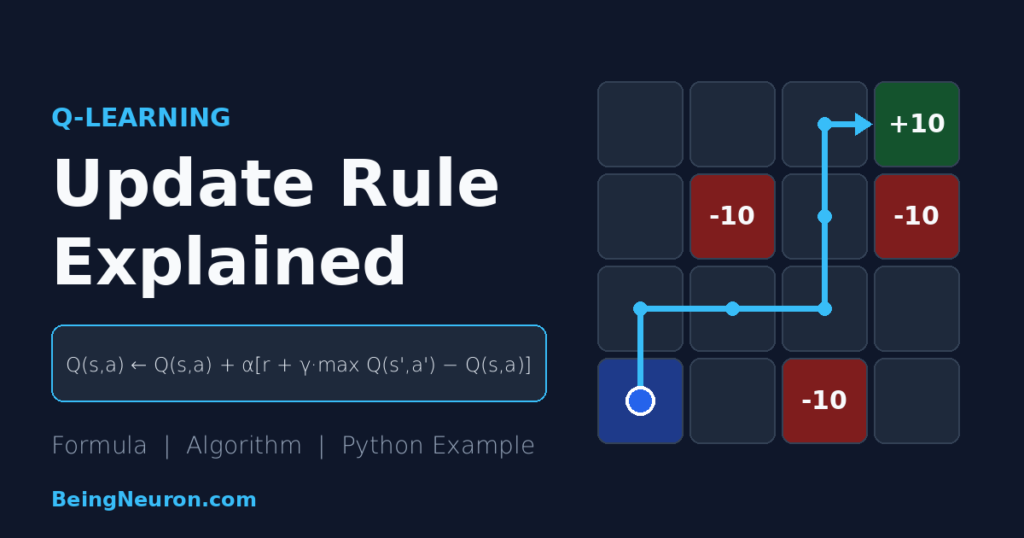
To see the update rule at work, we use a small GridWorld. The agent must travel from the bottom-left corner to the top-right corner while avoiding three pits.
| (0,0) | (0,1) | (0,2) | GOAL +10 |
| (1,0) | PIT −10 |
(1,2) | PIT −10 |
| (2,0) | (2,1) | (2,2) | (2,3) |
| START (3,0) |
(3,1) | PIT −10 |
(3,3) |
- Layout: 16 cells, so 16 states. Pits at (1,1), (1,3) and (3,2).
- Actions: up, down, left, right. Moving off the grid leaves the agent in place.
- Rewards and penalties: −1 for every ordinary move (so long routes cost more), +10 for reaching the goal, −10 for entering a pit. Goal and pits end the episode.
- Starting state: the bottom-left cell (3,0).
- Goal state: the top-right cell (0,3).
The shortest safe route takes 6 moves, which earns 5 × (−1) + 10 = +5. That is the best possible return, and a well-trained agent should achieve it.
How learning progresses. At first every Q-value is 0, so the agent wanders almost randomly and often falls into pits. The first time it falls into a pit, the Q-value of that final move drops toward −10. The first time it reaches the goal, the last move’s value rises toward +10. After that, the update rule passes value backward: the move before the goal now has a good “max Q” in its target, so its value rises, then the move before that, and so on. Over many episodes, a trail of increasing Q-values leads from the start to the goal.
Try it below. Press Step a few times to watch individual updates with their real numbers, then Train 100 episodes and watch the arrows organise into a route.
Interactive demo: watch Q-Learning train an agent
The blue dot is the agent. Arrows show the best action the agent currently believes in. Press Step to see one single update, or Play to let it learn.
| State (row, col) | ↑ up | ↓ down | ← left | → right |
|---|
Latest update, with real numbers:
Average return of recent episodes (dashed green line: best possible return, +5)
Things to try: set α to 1.0 and notice how aggressively values jump. Set γ to 0.5 and notice that values near the start shrink, because distant rewards count for less. Press Test greedy policy after training to watch the agent follow its learned route without exploring.
Implementing Q-Learning in Python Using NumPy
Now the same agent as plain Python. This Q learning code uses only NumPy, with no reinforcement learning framework, so every step of the update rule stays visible. Copy the stages below, in order, into one file named q_learning_gridworld.py. I tested the complete script with NumPy 2.5 and Python 3.
Stage 1: Import libraries and set the seed
import numpy as np

SEED = 42  # makes every run reproducible
NumPy provides the Q-table array and the random number generator. A fixed seed means you get the same results every time you run the script.
Stage 2: Define the GridWorld environment
# Row 0 is the top row. Cells are written as (row, column).
N_ROWS, N_COLS = 4, 4
START = (3, 0)                      # bottom-left
GOAL = (0, 3)                       # top-right
PITS = {(1, 1), (1, 3), (3, 2)}     # obstacles: they end the episode with a penalty

STEP_REWARD = -1.0                  # cost of every ordinary move
GOAL_REWARD = 10.0
PIT_REWARD = -10.0
These constants describe the world: its size, the start and goal cells, the pits, and the reward values. Changing them lets you design your own environment.
Stage 3: Define states and actions
ACTIONS = ["up", "down", "left", "right"]
ARROWS = ["↑", "↓", "←", "→"]
MOVES = [(-1, 0), (1, 0), (0, -1), (0, 1)]   # (row change, column change)

N_STATES = N_ROWS * N_COLS          # 16 states, numbered 0..15
N_ACTIONS = len(ACTIONS)            # 4 actions

def to_state(cell):
    """Convert (row, col) to a single state number."""
    row, col = cell
    return row * N_COLS + col

def to_cell(state):
    """Convert a state number back to (row, col)."""
    return divmod(state, N_COLS)

def step(state, action):
    """The environment: apply an action and return (next_state, reward, done)."""
    row, col = to_cell(state)
    d_row, d_col = MOVES[action]
    new_row, new_col = row + d_row, col + d_col

    # Moving off the grid leaves the agent where it is
    if not (0 <= new_row < N_ROWS and 0 <= new_col < N_COLS):
        new_row, new_col = row, col

    next_cell = (new_row, new_col)
    if next_cell == GOAL:
        return to_state(next_cell), GOAL_REWARD, True
    if next_cell in PITS:
        return to_state(next_cell), PIT_REWARD, True
    return to_state(next_cell), STEP_REWARD, False
The Q-table needs states as row numbers, so to_state flattens (row, column) into a single index. The step function is the environment: it takes a state and an action and returns the next state, the reward, and a done flag that is True when the episode has ended (goal or pit).
Stage 4: Initialize the Q-table
def create_q_table():
    return np.zeros((N_STATES, N_ACTIONS))
One row per state, one column per action, all zeros. The agent knows nothing yet.
Stage 5: Epsilon-greedy action selection
def choose_action(q_table, state, epsilon, rng):
    if rng.random() < epsilon:
        return int(rng.integers(N_ACTIONS))                 # explore: random action
    best_actions = np.flatnonzero(q_table[state] == q_table[state].max())
    return int(rng.choice(best_actions))                    # exploit: best action, ties broken randomly
With probability epsilon the function returns a random action. Otherwise it finds the action(s) with the highest Q-value. Ties matter early in training, when every value is 0, so the code picks randomly among tied actions instead of always choosing “up”.
Stage 6: The Q-Learning update rule
def update_q_value(q_table, state, action, reward, next_state, done, alpha, gamma):
    current_q = q_table[state, action]
    if done:
        target = reward                                     # terminal state: no future reward
    else:
        target = reward + gamma * np.max(q_table[next_state])
    td_error = target - current_q
    q_table[state, action] = current_q + alpha * td_error
    return td_error
This function is the formula, line by line. current_q is Q(s, a). The target is r + γ · max Q(s′, a′), except when done is true, where there is no future and the target is just the reward. td_error is target minus current value, and the last line adds α times that error. Nothing is hidden inside a library.
Stage 7: Train the agent
def train(episodes=500, alpha=0.1, gamma=0.9,
          epsilon_start=1.0, epsilon_min=0.05, epsilon_decay=0.99,
          max_steps=100, seed=SEED):
    rng = np.random.default_rng(seed)
    q_table = create_q_table()
    epsilon = epsilon_start
    episode_returns = []

    for _ in range(episodes):
        state = to_state(START)
        total_reward = 0.0

        for _ in range(max_steps):
            action = choose_action(q_table, state, epsilon, rng)
            next_state, reward, done = step(state, action)
            update_q_value(q_table, state, action, reward, next_state, done, alpha, gamma)
            total_reward += reward
            state = next_state
            if done:                                        # goal or pit reached: end the episode
                break

        episode_returns.append(total_reward)
        epsilon = max(epsilon_min, epsilon * epsilon_decay) # explore less as training goes on

    return q_table, episode_returns
This is the algorithm from earlier, in code. The outer loop runs episodes, and the inner loop runs steps inside one episode. The max_steps limit stops an episode that wanders forever. When done is true, the inner loop breaks, which is how terminal states end an episode. After each episode, epsilon shrinks by 1% until it reaches its floor of 0.05.
Stage 8: Evaluate the trained agent
def evaluate(q_table, max_steps=50):
    state = to_state(START)
    path = [to_cell(state)]
    total_reward = 0.0
    for _ in range(max_steps):
        action = int(np.argmax(q_table[state]))
        state, reward, done = step(state, action)
        path.append(to_cell(state))
        total_reward += reward
        if done:
            break
    return path, total_reward
Evaluation uses the greedy policy: no random actions and no learning. The function follows the best Q-value from the start cell and records the path and total reward.
Stage 9: Display the learned policy
def print_policy(q_table):
    for row in range(N_ROWS):
        symbols = []
        for col in range(N_COLS):
            cell = (row, col)
            if cell == GOAL:
                symbols.append("G")
            elif cell in PITS:
                symbols.append("X")
            else:
                symbols.append(ARROWS[int(np.argmax(q_table[to_state(cell)]))])
        print("  ".join(symbols))

if __name__ == "__main__":
    q_table, returns = train()

    for first in range(0, 500, 100):
        average = np.mean(returns[first:first + 100])
        print(f"Episodes {first + 1:>3}-{first + 100:>3}: average return = {average:6.2f}")

    path, total = evaluate(q_table)
    print("\nGreedy path:", path)
    print("Total reward:", total)

    print("\nLearned policy:")
    print_policy(q_table)

    print("\nQ-values at the start cell (up, down, left, right):",
          np.round(q_table[to_state(START)], 2))
The final stage prints one arrow per cell (G for the goal, X for pits) and then runs everything. Running the script produces this output:
Episodes   1-100: average return = -12.73
Episodes 101-200: average return =  -0.50
Episodes 201-300: average return =   2.45
Episodes 301-400: average return =   3.83
Episodes 401-500: average return =   2.97

Greedy path: [(3, 0), (2, 0), (2, 1), (2, 2), (1, 2), (0, 2), (0, 3)]
Total reward: 5.0

Learned policy:
→  →  →  G
↑  X  ↑  X
→  →  ↑  ←
↑  ↑  X  →

Q-values at the start cell (up, down, left, right): [ 1.81 -1.23 -1.01 -2.05]
Reading the results. The average training return climbs from −12.73 to a few points above zero as the agent stops falling into pits. It stays below the ideal +5 during training because ε never drops below 0.05, so the agent still takes occasional random moves. The greedy evaluation shows what it actually learned: a 6-move path with a total reward of +5.0, the best possible. The start cell’s best Q-value, 1.81, matches the value you get by working backward from the goal with γ = 0.9: 10, 8, 6.2, 4.58, 3.122, then 1.8098.
A note on the policy grid: arrows for cells the agent rarely visits, such as (3,3) or (2,3), are less reliable than arrows along the main route, because those states have received few updates. Also, exact numbers can differ slightly across NumPy versions because random number streams are not guaranteed identical between releases. In testing, 20 different seeds all reached the optimal return of +5.0.
Why Is Q-Learning an Off-Policy Algorithm?
A policy is the rule an agent uses to choose actions. Learning algorithms differ in whether they learn about the same policy they follow.
- On-policy learning evaluates and improves the policy the agent is actually using to act, including its exploratory moves.
- Off-policy learning evaluates one policy (the target policy) while following another (the behavior policy).
Q-learning is off-policy. Its behavior policy is epsilon-greedy, so it sometimes takes random actions. But its update target uses max Q(s′, a′), which assumes the agent will take the best action in the next state, whatever action it actually takes. In other words, the agent behaves exploratorily but learns the values of the greedy policy.
A simple example. The agent stands in cell (2,2) and, because ε triggered a random move, steps “down” into the pit at (3,2) instead of the best move. The next time it is in a cell next to a good state, the update uses the best next value, not the random move it actually made. So one unlucky exploratory step does not drag down the estimate of what a sensible agent could achieve from that state.
This has a famous consequence in the textbook “cliff walking” task. Q-learning learns the shortest route right along the cliff edge, which is optimal for a greedy agent, but while still exploring it occasionally falls off. SARSA, which is on-policy, learns a longer but safer path because its estimates include the risk of its own random moves.
Advantages and Disadvantages of Q-Learning
Advantages
- Model-free. It needs no knowledge of transition probabilities or reward rules, so it works when the environment is unknown.
- Simple to implement. The core is one update line and a table, as the Python code shows.
- Learns optimal policies under suitable conditions. In the tabular case, Q-values converge to the optimal values if every state-action pair is visited infinitely often and the learning rate is decreased appropriately. In practice you approximate these conditions.
- Off-policy flexibility. It can learn from exploratory behavior, and in principle from experience collected by a different policy.
Disadvantages
- Q-tables do not scale. The table grows with the number of states times the number of actions. Large or continuous state spaces make a table impossible.
- Slow in big problems. Information spreads one step at a time, so long tasks need many episodes.
- Exploration is hard. Epsilon-greedy explores blindly. When rewards are rare, the agent may rarely find a reward to learn from.
- Sensitive to hyperparameters. Poor choices of α, γ, and the ε schedule can slow or break learning.
- Overestimation. Taking a max over noisy estimates tends to bias values upward. Variants such as Double Q-learning were designed to reduce this.
Applications of Q-Learning in AI
Q-learning in AI is best understood as a foundation. Plain tabular Q-learning is mainly used for learning and for small problems, while its ideas power larger systems. The table separates what is well established from what is illustrative or research-stage.
| Area | Status | Notes |
|---|---|---|
| Game-playing agents | Established | Tabular Q-learning is a standard teaching benchmark on small games. Deep Q-Networks, a neural network extension, learned to play many Atari games from screen pixels (Mnih et al., Nature, 2015). |
| Navigation | Established in research and teaching | Grid and maze navigation, like this article’s example, is the classic use. Real-world navigation usually needs far larger or continuous state spaces. |
| Robotics | Research | Q-learning has been studied for simple robot navigation and control tasks, often in simulation. Real robot control usually uses deep or policy-based RL instead. |
| Traffic signal optimization | Research, mostly simulation | Researchers have used Q-learning variants to adjust signal timing in simulated traffic networks. Treat these as studies, not proven deployments. |
| Resource allocation | Illustrative | Problems like allocating network channels or computing resources can be framed as states, actions, and rewards, and Q-learning has been explored for them. It is a plausible fit, not a standard solution. |
For a wider survey of where reinforcement learning is used, see Applications of Reinforcement Learning: 10 Real-World Examples.
Q-Learning vs SARSA
SARSA is the closest relative of Q-learning. Its name comes from the tuple it uses for each update: State, Action, Reward, next State, next Action. The two differ in one term of the update.
| Aspect | Q-Learning | SARSA |
|---|---|---|
| Learning approach | Model-free temporal difference learning | Model-free temporal difference learning |
| Policy type | Off-policy | On-policy |
| Update equation | Q(s,a) ← Q(s,a) + α [ r + γ maxa′ Q(s′,a′) − Q(s,a) ] | Q(s,a) ← Q(s,a) + α [ r + γ Q(s′,a′) − Q(s,a) ] |
| Action selection in the target | Uses the best next action (max), regardless of what is actually chosen | Uses the next action a′ that the policy actually selects |
| Learning behavior | Learns the greedy (optimal) policy; can take risky routes while exploring | Learns the value of the exploring policy; tends to prefer safer routes |
When to use which. Choose Q-learning when you want the optimal greedy policy and mistakes during training are cheap, as in simulation. Choose SARSA when the agent’s behavior during learning matters, for example when exploratory mistakes are costly and you want the agent to account for its own exploration risk.
Q-Learning vs Deep Q-Learning
Tabular Q-learning and Deep Q-Learning share the same core idea, but they store values very differently. Deep Q-Learning, introduced through the Deep Q-Network (DQN), is not the same algorithm as ordinary tabular Q-learning. It is an extension built for problems the table cannot handle.
| Aspect | Tabular Q-Learning | Deep Q-Learning (DQN) |
|---|---|---|
| Value storage | Q-table: one entry per state-action pair | Neural network that outputs a Q-value for each action |
| State space | Small and discrete | Large, such as images or continuous values |
| Generalization | None: each state is learned separately | Similar states share what the network learned |
| Stability | Simple and well understood | Needs extra techniques to train stably |
- Function approximation. Instead of a table, a neural network approximates Q(s, a). Because the network generalizes, it can handle states it has never seen exactly. If you want background on such networks, see Multilayer Perceptron.
- Experience replay. DQN stores past transitions (s, a, r, s′) in a buffer and trains on random samples from it. This breaks the correlation between consecutive steps and reuses data efficiently.
- Target networks. DQN computes the target r + γ max Q(s′, a′; θ⁻) with a separate copy of the network whose weights θ⁻ are updated only occasionally. This keeps the target from shifting with every training step.
In short: the update idea is the same, a target built from reward plus discounted best next value. But DQN trains a network by gradient descent to move its prediction toward that target, while tabular Q-learning edits one table cell directly.
Frequently Asked Questions
What is Q-Learning in simple terms?
Q-learning is a way for an agent to learn good behavior by trial and error. It keeps a score for every action in every situation, updates the score after each step using the reward it received, and eventually picks the highest-scoring action.
What is the Q-Learning update rule?
It is the equation the agent uses to revise a score after each step: it moves the old Q-value toward a target made of the immediate reward plus the discounted best Q-value of the next state. The size of the move is set by the learning rate.
What is the formula for Q-Learning?
Q(s, a) ← Q(s, a) + α [ r + γ · maxa′ Q(s′, a′) − Q(s, a) ], where α is the learning rate, γ is the discount factor, r is the reward, and s′ is the next state.
What is a Q-value in reinforcement learning?
A Q-value is the expected total future reward of taking a particular action in a particular state and then acting well afterwards. Higher Q-values mark better actions.
Why is Q-Learning considered off-policy?
Because it learns the value of the greedy policy (through the max in its target) while the agent actually behaves with an exploratory, epsilon-greedy policy. The policy it learns about differs from the policy it follows.
What is the difference between Q-Learning and SARSA?
Q-learning updates toward the best possible next action (off-policy), while SARSA updates toward the next action actually taken (on-policy). As a result, Q-learning learns the optimal greedy policy and SARSA learns a policy that accounts for its own exploration.
Can Q-Learning be implemented using Python?
Yes. The tabular algorithm needs only a NumPy array for the Q-table, an environment with a step function, and the update rule. The full working example above uses about 100 lines of plain Python and NumPy.
Where to Go Next
You now have the full picture: the formula, the arithmetic behind it, the algorithm, and a working agent. A good next step is to experiment with the code: change the pit positions, try different α, γ, and ε-decay values, or add a wall. To place Q-learning within the larger field, read Reinforcement Learning vs Supervised Learning, and when tables stop being enough, the natural next topic is Deep Q-Networks.