Support Vector Machines (SVM): How They Work

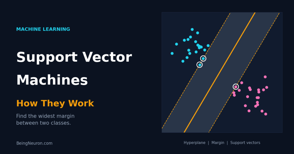
A Support Vector Machine (SVM) classifies data by finding the boundary that separates two classes with the widest possible gap. Of all the lines that could split the data, SVM picks the one that stays farthest from the nearest training points on each side. That choice makes it a strong, well-founded classifier for small and medium datasets, particularly when the number of features is large.

This guide explains how SVMs work from the geometry up: hyperplanes, margins, support vectors, the soft margin and the C parameter, and the kernel trick that lets a linear method draw curved boundaries. You will then build SVM models on the Breast Cancer dataset with scikit-learn, compare kernels, tune C and gamma, and learn how to avoid the usual mistakes.

What Is a Support Vector Machine?

SVM is a supervised learning algorithm used for classification (SVC), regression (SVR), and outlier detection (OneClassSVM). In its classification form it answers one question: which dividing boundary is the safest?

Imagine two groups of points on a sheet of paper. Many straight lines separate them perfectly. A line that squeezes between two points is fragile, because a small shift in the data moves a point to the wrong side. SVM chooses the line with the largest distance to the closest points of both classes. That distance is the margin, and a larger margin usually means better generalization to new data.

Core Concepts: Hyperplane, Margin, and Support Vectors

• Hyperplane: the decision boundary. In 2 dimensions it is a line, in 3 dimensions a plane, and in higher dimensions a flat subspace called a hyperplane.
• Margin: the empty band on both sides of the hyperplane, bounded by the nearest training points.
• Support vectors: the training points that lie exactly on the margin boundary. They are the only points that determine the hyperplane. Remove any other point and the boundary does not move.

Hyperplane x1 + x2 = 5 with margins x1 + x2 = 4 and x1 + x2 = 6. Support vectors are (3,3), (4,2), (2,2) and (3,1).A maximum-margin classifier in 2DHyperplaneFeature 1Feature 2Worked example: w = (1, 1), b = −5Decision value f(x) = x₁ + x₂ − 5(3, 3): f = +1, on the positive margin(4, 2): f = +1, on the positive margin(2, 2): f = −1, on the negative margin(3, 1): f = −1, on the negative marginMargin width = 2 / ||w|| = 2 / 1.41 = 1.41Circled points are support vectors.Other points could move without changing the line.

The Mathematics of SVM

The Decision Function

f(x) = w · x + b,   predicted class = sign(f(x))

• x is the feature vector of one example.
• w is the weight vector. It is perpendicular to the hyperplane and sets its orientation.
• b is the bias (intercept), which shifts the hyperplane away from the origin.
• The dot product w · x multiplies matching entries and adds them: for w = (1, 1) and x = (3, 3) it is 1·3 + 1·3 = 6.

With labels y = +1 or −1, a point is correctly classified when y(w · x + b) > 0. In the example in Figure 1, the point (3, 3) gives 3 + 3 − 5 = 1.

Margin Width

The margin boundaries are the lines where f(x) = +1 and f(x) = −1. The distance between them is

margin = 2 / ||w||

where ||w|| is the length of w: √(w₁² + w₂² + …). For w = (1, 1), ||w|| = 1.41 and the margin is 1.41. A shorter w means a wider margin.

The Optimization Problem (Hard Margin)

Maximizing the margin is the same as minimizing ||w||, which is done through its square for convenience:

minimize ½||w||²   subject to   y_i(w · x_i + b) ≥ 1   for every training point i

The constraint forces every point to sit on or outside its margin boundary. This is the hard margin SVM, and it only has a solution when the classes are perfectly linearly separable. It is also very sensitive to outliers, because a single mislabeled point can make the problem unsolvable or tilt the line badly.

The Soft Margin and the C Parameter

Real data overlaps. The soft margin SVM allows some points to violate the margin, at a price:

minimize ½||w||² + C Σ_i ξ_i   subject to   y_i(w · x_i + b) ≥ 1 − ξ_i,   ξ_i ≥ 0

• ξ_i (xi) is the slack of point i: zero if the point is correct and outside the margin, between 0 and 1 if it is inside the margin but correctly classified, and above 1 if it is misclassified.
• C is the penalty on total slack. It sets the trade-off between a wide margin and few violations.

Equivalently, the soft-margin SVM minimizes the hinge loss, max(0, 1 − y_if(x_i)), plus a regularization term. Points beyond the margin contribute zero loss, which is why only support vectors matter.

Small C: wide margin with two points inside. Large C: tilted line with a narrow margin.Small C: wide margin, more support vectorsLarge C: narrow margin, fits every pointSame data, two values of C. Large C risks overfitting to the two closest points.Schematic illustration; see Figure 3 for measured results.

The Kernel Trick: Non-Linear Classification

A single straight hyperplane cannot separate every dataset. The classic fix is to map the data into a higher-dimensional space where it is linearly separable. The example below uses one feature x. The orange class sits at −1, 0, and 1, and the blue class sits at −3, −2, 2, and 3. No single cut on the number line separates them. Add a second feature x², and a horizontal line does.

Points at -3,-2,2,3 are blue and -1,0,1 are orange. After adding x squared, the line x squared = 2.5 separates them.Original space: not separableFeature space (x, x²): separable-3-2-10123Any single cut puts both classes on one side.x² = 2.5940x (horizontal), x² (vertical)

Computing the new coordinates explicitly becomes expensive or impossible in high dimensions. The kernel trick avoids it. The SVM training and prediction formulas depend on the data only through dot products between pairs of points. A kernel function K(x, x′) returns the dot product in the lifted space directly, without ever building that space. The prediction becomes:

f(x) = Σ_{i in support vectors} α_i y_i K(x_i, x) + b

Here α_i are learned coefficients (nonzero only for support vectors), y_i are the labels, and x_i are the support vectors. Common kernels:

Kernel	Formula	Use it when
Linear	K = x · x′	Many features, text data, or nearly linear classes
Polynomial	K = (γ x · x′ + r)d	Interactions of known degree d matter
RBF (Gaussian)	K = exp(−γ ||x − x′||²)	General-purpose default for non-linear data
Sigmoid	K = tanh(γ x · x′ + r)	Rarely; behaves like a neural network layer

In the RBF kernel, γ (gamma) controls how far one training point’s influence reaches. A small γ gives each point a wide influence and a smooth boundary. A large γ gives each point a small, local influence and a wiggly boundary that can memorize the training set. The RBF kernel value is 1 for identical points and falls toward 0 as points move apart.

Key Hyperparameters

• C (default 1.0): penalty for margin violations. Increase it to fit the training data more tightly; decrease it for a wider margin and more regularization.
• kernel (default "rbf"): "linear", "poly", "rbf", or "sigmoid".
• gamma (default "scale"): reach of a single point for RBF, poly, and sigmoid kernels. "scale" uses 1 / (number of features × variance of X).
• degree (default 3): polynomial degree, used only by the poly kernel.
• class_weight: set to "balanced" for imbalanced classes.
• probability (default False): enables predict_proba, but slows training because it runs an internal cross-validation.

SVM in Python with Scikit-Learn

The task: classify breast tumors as malignant or benign from 30 cell-nucleus measurements (569 samples). SVM uses distances and dot products, so it needs feature scaling. On the Wine dataset, the same default SVM scored 66.3% cross-validated accuracy on raw features and 98.3% after standardization.

Step 1: Load and split the data

from sklearn.datasets import load_breast_cancer
from sklearn.model_selection import train_test_split

X, y = load_breast_cancer(return_X_y=True)
X_train, X_test, y_train, y_test = train_test_split(
    X, y, test_size=0.25, random_state=42, stratify=y
)

Step 2: Compare kernels inside a pipeline

from sklearn.pipeline import make_pipeline
from sklearn.preprocessing import StandardScaler
from sklearn.svm import SVC

for kernel in ["linear", "rbf", "poly"]:
    pipe = make_pipeline(StandardScaler(), SVC(kernel=kernel))
    pipe.fit(X_train, y_train)
    n_sv = len(pipe[-1].support_)          # number of support vectors
    print(f"{kernel:7s} test accuracy = {pipe.score(X_test, y_test):.3f}, "
          f"support vectors = {n_sv}")

Output:

linear  test accuracy = 0.986, support vectors = 34
rbf     test accuracy = 0.979, support vectors = 96
poly    test accuracy = 0.902, support vectors = 136

pipe[-1] selects the last pipeline step, the SVC. The attribute support_ holds the indices of the support vectors. Two lessons appear in this output. First, the linear kernel wins: this dataset is nearly linearly separable, so a more flexible kernel adds nothing. Second, fewer support vectors (34 of 426 training points) indicate a simpler, cleaner boundary. Always test a linear kernel before assuming you need a non-linear one.

Step 3: See what C does

for C in [0.01, 0.1, 1, 10, 100]:
    pipe = make_pipeline(StandardScaler(), SVC(C=C)).fit(X_train, y_train)
    print(f"C={C:<6} SVs={len(pipe[-1].support_):3d}  "
          f"train={pipe.score(X_train, y_train):.3f}  "
          f"test={pipe.score(X_test, y_test):.3f}")

Output:

C=0.01   SVs=320  train=0.627  test=0.629
C=0.1    SVs=191  train=0.962  test=0.937
C=1      SVs= 96  train=0.979  test=0.979
C=10     SVs= 78  train=0.993  test=0.979
C=100    SVs= 67  train=1.000  test=0.944

C values 0.01, 0.1, 1, 10, 100. Train accuracy 0.627, 0.962, 0.979, 0.993, 1.000. Test accuracy 0.629, 0.937, 0.979, 0.979, 0.944. Support vectors 320, 191, 96, 78, 67.Accuracy vs CSupport vectors vs C1.00.90.80.70.60.010.1110100test 0.944trainC (log scale)3201919678670.010.1110100C (log scale)Test accuracy peaks at C = 1 to 10; at C = 100 training accuracy hits 1.000 while test accuracy falls to 0.944.

The number of support vectors falls as C grows, because the margin narrows and fewer points sit inside or on it. The training accuracy keeps climbing to 1.000 while test accuracy drops from 0.979 to 0.944: the signature of overfitting.

Step 4: Tune C and gamma together

from sklearn.model_selection import GridSearchCV

param_grid = {"svc__C": [0.1, 1, 10, 100],
              "svc__gamma": [0.001, 0.01, 0.1, 1]}

search = GridSearchCV(make_pipeline(StandardScaler(), SVC()), param_grid, cv=5)
search.fit(X_train, y_train)

print(search.best_params_)
print("Best CV accuracy:", round(search.best_score_, 3))
print("Test accuracy:   ", round(search.score(X_test, y_test), 3))

Output:

{'svc__C': 10, 'svc__gamma': 0.001}
Best CV accuracy: 0.977
Test accuracy:    0.979

The best RBF model uses a large C with a very small gamma, which pushes it toward a nearly linear boundary: the search rediscovered what Step 2 showed. Tune C and gamma on a logarithmic grid (powers of 10), because their effects are multiplicative.

Step 5: A genuinely non-linear problem

Two interleaved half-circles (make_moons) cannot be split by a line. Here the kernel choice matters.

from sklearn.datasets import make_moons
from sklearn.model_selection import cross_val_score

Xm, ym = make_moons(n_samples=300, noise=0.25, random_state=0)

models = {
    "linear": SVC(kernel="linear"),
    "poly (degree 3)": SVC(kernel="poly", degree=3),
    "rbf (gamma=1)": SVC(kernel="rbf", gamma=1),
}
for name, model in models.items():
    print(f"{name:16s} {cross_val_score(model, Xm, ym, cv=5).mean():.3f}")

Output:

linear           0.837
poly (degree 3)  0.860
rbf (gamma=1)    0.957

Breast Cancer test accuracy: linear 0.986, RBF 0.979, poly 0.902. Moons 5-fold CV accuracy: linear 0.837, RBF 0.957, poly 0.860.The best kernel depends on the data00.51.00.9860.9790.9020.8370.9570.860LinearRBFPolyLinearRBFPolyBreast Cancer (test accuracy)Moons (5-fold CV accuracy)

Step 6: Practical extras

pipe = make_pipeline(StandardScaler(), SVC(kernel="rbf", C=10, gamma=0.001))
pipe.fit(X_train, y_train)

# Signed distance to the hyperplane (positive = class 1)
scores = pipe.decision_function(X_test[:3])

# Support vectors per class
print(pipe[-1].n_support_)

# Imbalanced data
SVC(class_weight="balanced")

# Probability estimates (slower training)
SVC(probability=True)

# Large datasets: linear SVM with a faster solver
from sklearn.svm import LinearSVC
LinearSVC(C=1.0, max_iter=10000)

decision_function returns the value of f(x): its sign gives the class and its size gives the confidence, with 0 meaning on the hyperplane and ±1 on the margin.

Multi-Class SVM and SVM Regression

SVM is inherently a binary classifier. For more than two classes, scikit-learn’s SVC trains one classifier for every pair of classes (one-vs-one) and combines their votes, which takes K(K − 1)/2 classifiers for K classes. LinearSVC uses one-vs-rest, training K classifiers, each separating one class from all others.

Support Vector Regression (SVR) flips the idea: instead of a gap that excludes points, it fits a tube of width ε (epsilon) around the prediction and ignores errors inside the tube. Only points outside the tube become support vectors. Use SVR(kernel="rbf", C=..., epsilon=...) with scaled features.

Advantages and Disadvantages of SVM

Advantages

• Effective in high-dimensional spaces, even when features outnumber samples.
• Memory efficient at prediction time: only support vectors are stored.
• Flexible through kernels, so it handles linear and non-linear problems.
• Maximum-margin training gives strong generalization on small and medium datasets.

Disadvantages and Limitations

• Kernel SVM training time grows between O(n²) and O(n³) with the number of samples, so it becomes impractical beyond roughly 100,000 samples. Use LinearSVC or SGDClassifier there.
• Requires feature scaling.
• Sensitive to the choice of kernel, C, and gamma.
• Does not output probabilities natively; probability=True adds cost and the probabilities are approximations.
• Hard to interpret with non-linear kernels. Only the linear kernel exposes usable coefficients (coef_).
• Performs poorly when classes overlap heavily and the data is very noisy.

Common Mistakes and How to Fix Them

Not scaling the features

The most damaging mistake: 66.3% vs 98.3% on the Wine data. Put StandardScaler in a pipeline.

Assuming the RBF kernel is always best

Figure 5 shows a linear kernel beating RBF and polynomial on the Breast Cancer data. Start with linear as a baseline, particularly with many features.

Setting gamma too high

A large gamma makes each point’s influence tiny, so the model memorizes training data: near-perfect training score, poor test score. Grid-search gamma on a log scale.

Using the default C without tuning

Figure 4 shows the range from underfitting to overfitting across C alone.

ConvergenceWarning from LinearSVC

ConvergenceWarning: Liblinear failed to converge usually means unscaled features or too few iterations. Scale the data and raise max_iter.

Training kernel SVM on huge datasets

If fit() takes hours, switch to LinearSVC, SGDClassifier(loss="hinge"), or subsample the data.

Turning on probability=True by default

It multiplies training time by several times. Use decision_function unless you really need calibrated probabilities.

Ignoring class imbalance

A margin that favors the majority class gives high accuracy and poor recall on the rare class. Use class_weight="balanced" and evaluate recall and F1.

Real-World Applications of SVM

• Text classification: spam filtering and topic labeling use linear SVMs on sparse word-count features.
• Bioinformatics: classifying tumors or proteins from gene-expression data, where features far outnumber samples.
• Image recognition: classic digit and face recognition pipelines used SVMs on extracted features.
• Medical diagnosis: separating malignant from benign cases, as in the tutorial.
• Anomaly detection: OneClassSVM learns the boundary of normal data and flags points outside it.

Related reading on BeingNeuron: Feature Scaling: Normalization vs Standardization, K-Nearest Neighbors (KNN) Algorithm Explained, Cross-Validation: K-Fold Explained, and Gradient Boosting: How It Works.

Frequently Asked Questions

How does a Support Vector Machine work?

It finds the hyperplane that separates the classes with the largest margin. The points closest to the boundary, the support vectors, define it. With kernels, it can also draw curved boundaries.

What are support vectors in SVM?

Support vectors are the training points on or inside the margin. They are the only points that influence the position of the hyperplane. All other points can be removed without changing the model.

What does the C parameter do in SVM?

C sets the penalty for margin violations. A small C allows more violations and produces a wider margin (more regularization). A large C punishes violations heavily and produces a narrower margin that fits the training data more closely.

What is the kernel trick?

It computes dot products in a higher-dimensional feature space without building that space explicitly. This lets a linear SVM separate data that is not linearly separable in the original features.

Which kernel should I use?

Try linear first, particularly for high-dimensional or text data. Use RBF for general non-linear problems. Choose between them with cross-validation.

What is gamma in SVM?

Gamma controls the reach of a single training point in RBF, polynomial, and sigmoid kernels. Low gamma means far reach and a smooth boundary. High gamma means local influence and a complex boundary that can overfit.

Does SVM require feature scaling?

Yes. Margins and kernels depend on distances, so unscaled features distort them. Standardize features before training.

Is SVM good for large datasets?

Kernel SVM scales poorly with the number of samples. For large datasets use LinearSVC or stochastic gradient descent with hinge loss, or consider tree ensembles.

Can SVM do multi-class classification?

Yes, by combining several binary classifiers: one-vs-one in SVC and one-vs-rest in LinearSVC.

SVM vs logistic regression: what is the difference?

Both give linear boundaries by default. Logistic regression minimizes log loss and outputs calibrated probabilities. SVM maximizes the margin using hinge loss and depends only on support vectors. SVM gains power through kernels.

Conclusion

An SVM places the decision boundary where it is safest: as far as possible from the closest points of each class. Soft margins (controlled by C) let it cope with overlap, and kernels (controlled by gamma and the kernel type) let it bend the boundary. In practice, the recipe is short: standardize features, test a linear kernel first, move to RBF only when the data demands it, tune C and gamma on a log grid with cross-validation, and use linear solvers when the dataset grows large.

To validate those tuning choices fairly, continue with K-Fold Cross-Validation.