K-Nearest Neighbors (KNN) Algorithm Explained

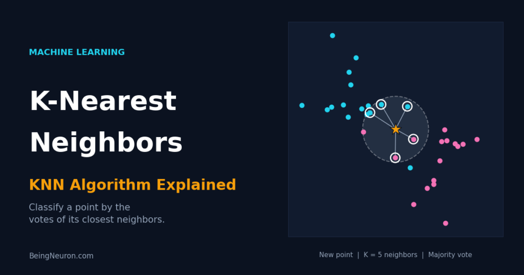
The K-Nearest Neighbors (KNN) algorithm predicts the label of a new data point by looking at the k most similar points in the training data and letting them vote. It has no training phase in the usual sense and no equations to fit, which makes it the easiest supervised learning algorithm to understand and a strong baseline for classification and regression.

This guide covers how KNN works, the distance formulas behind it, how to choose k, why feature scaling is essential, and what happens to KNN in high dimensions. You will also build a complete scikit-learn classifier on the Breast Cancer dataset, tune it with grid search, and learn the mistakes that most often break KNN models.

What Is the K-Nearest Neighbors Algorithm?

KNN is a supervised learning algorithm: it learns from examples that already have labels. It is built on one assumption: similar things are close to each other. If most of the five patients most similar to a new patient have a benign tumor, the new patient probably does too.

Three terms describe KNN precisely:

• Instance-based: the model is the training data itself. There are no learned weights or coefficients.
• Lazy learner: fit() only stores the data. All the work happens at prediction time, when distances are computed.
• Non-parametric: KNN makes no assumption about the shape of the data distribution, so it can fit very irregular decision boundaries.

How KNN Works Step by Step

1. Choose k, the number of neighbors to consult.
2. Measure the distance from the new point to every training point.
3. Sort the training points by distance and keep the k closest.
4. Vote. For classification, the most common class among the neighbors wins. For regression, average the neighbors’ target values.

A Worked Example You Can Verify by Hand

Six training points with two features each, and a query point Q = (5, 4):

Point	Class	Distance to Q (Euclidean)	Rank
(6, 5)	Blue	√(1² + 1²) = 1.41	1
(3, 2)	Red	√(2² + 2²) = 2.83	2
(2, 3)	Red	√(3² + 1²) = 3.16	3
(7, 7)	Blue	√(2² + 3²) = 3.61	4 (tie)
(8, 6)	Blue	√(3² + 2²) = 3.61	4 (tie)
(1, 1)	Red	√(4² + 3²) = 5.00	6

Query point at (5,4). The three nearest neighbors are (6,5) blue, (3,2) red and (2,3) red, so k=3 predicts red.Neighborhood of the query point (k = 3)Q (5, 4)Feature 1Feature 2Vote among the 3 nearest1st: (6, 5) Blue, d = 1.412nd: (3, 2) Red, d = 2.833rd: (2, 3) Red, d = 3.16Result by kk = 1: Blue (1 vote to 0)k = 3: Red (2 votes to 1)k = 5: Blue (3 votes to 2)The prediction flips as k changes.

This tiny example shows the central design decision in KNN: the answer depends on k. With k = 1 the query is Blue. With k = 3 two of the three neighbors are Red, so it is Red. With k = 5 the neighbors are Blue, Red, Red, Blue, Blue, so Blue wins 3 to 2.

Distance Metrics Used in KNN

“Nearest” requires a definition of distance. The right choice depends on the data type.

Euclidean Distance

d(a, b) = √( Σ_i=1..n (a_i − b_i)² )

Here a and b are two data points, n is the number of features, and a_i, b_i are their values on feature i. It is the straight-line distance and the default in scikit-learn.

Manhattan Distance

d(a, b) = Σ_i=1..n |a_i − b_i|

The sum of absolute differences, like walking along city blocks. It is less sensitive to a single large difference and often works better with many features.

Minkowski Distance

d(a, b) = ( Σ_i |a_i − b_i|^p )^1/p

A general form where p controls the shape: p = 1 gives Manhattan and p = 2 gives Euclidean. In scikit-learn the default is metric="minkowski" with p=2, which equals Euclidean.

Other Metrics

• Cosine distance: compares the angle between vectors, ignoring length. It suits text represented as word counts or embeddings.
• Hamming distance: counts the positions where two categorical vectors differ.

Between (0,0) and (3,4) the Euclidean distance is 5 and the Manhattan distance is 7.A (0, 0)B (3, 4)Euclidean = 5Manhattan = 7Between A and BEuclidean = √(3² + 4²) = √25 = 5Manhattan = |3| + |4| = 7Minkowski with exponent pp = 1 gives Manhattan, p = 2 gives EuclideanBoth metrics are valid; they rank neighbors differently.

How to Choose the Value of K

k controls the bias-variance trade-off:

• Small k (such as 1): the decision boundary follows every training point, including noise. The model has low bias and high variance and overfits.
• Large k: the boundary becomes smooth, but the model starts to ignore real local patterns. It has high bias and underfits. In the extreme case where k equals the number of training points, KNN always predicts the majority class.

Schematic panels: k=1 overfits with islands, k=5 balanced, k=25 oversmoothed.k = 1: overfitsk = 5: balancedk = 25: oversmoothedSchematic illustration of boundary shape. Pink = predicted red, light blue = predicted blue.

Measured Effect of k on Real Data

The chart below uses the Breast Cancer Wisconsin dataset (569 patients, 30 features, standardized). It shows training accuracy, test accuracy, and 5-fold cross-validation accuracy for increasing k.

Training, test and cross-validation accuracy for k = 1, 3, 5, 7, 11, 15, 25, 41.Accuracy vs k (Breast Cancer, standardized features)1.000.990.970.950.93135711152541k (number of neighbors)TrainingTest5-fold cross-validation (training set)

Practical rules for choosing k:

• Use odd values of k for two-class problems to avoid tied votes.
• Search k with cross-validation (see the grid search below), not with test accuracy. A common starting range is 1 to 30.
• A rough starting point is √n, where n is the number of training samples, but treat it only as a guess.

Weighted KNN and KNN Regression

Weighted KNN gives closer neighbors more influence. Each neighbor’s vote is multiplied by w = 1/d, where d is its distance to the query. In scikit-learn set weights="distance". It helps when classes overlap or when the neighbor set contains a few very distant points.

KNN regression predicts a number by averaging the neighbors’ targets:

ŷ = (1/k) Σ_{i in neighbors} y_i

Here ŷ is the prediction and y_i is the target value of the i-th neighbor. For example, predicting a house price from the five most similar houses means averaging their five sale prices. Use KNeighborsRegressor.

Why Feature Scaling Is Essential for KNN

KNN is built on distances, so a feature measured in large units overwhelms the rest. In the feature scaling guide, the same KNN model on the Wine dataset scored 69.1% accuracy with raw features and 94.9% after standardization. Always scale numeric features before KNN, and fit the scaler on the training data only.

The Curse of Dimensionality

KNN works best with a moderate number of informative features. As the number of dimensions grows, distances between points become almost identical, so “nearest” loses its meaning. A simple experiment shows this. Take 1,000 random points in a unit hypercube, pick a random query, and measure the relative contrast (farthest distance minus nearest distance, divided by nearest distance):

Relative contrast for 5, 10, 20, 50, 100, 500 and 1000 dimensions: 7.40, 2.41, 1.24, 0.90, 0.38, 0.16, 0.11.Relative contrast (farthest minus nearest) / nearest7.402.411.240.900.380.160.1151020501005001000Number of dimensions (1,000 uniform random points, one random query)

This is a property of random uniform data. Real data usually lies on a lower-dimensional structure, so KNN can still work with many features, but irrelevant features hurt it directly. Mitigations: select features, apply PCA, or switch to a model that learns feature importance, such as tree ensembles.

KNN in Python with Scikit-Learn

The task: classify breast tumors as malignant or benign from 30 measurements of cell nuclei (569 samples).

Step 1: Load the data and split

from sklearn.datasets import load_breast_cancer
from sklearn.model_selection import train_test_split

data = load_breast_cancer()
X, y = data.data, data.target     # 0 = malignant, 1 = benign

X_train, X_test, y_train, y_test = train_test_split(
    X, y, test_size=0.25, random_state=42, stratify=y
)
print(X_train.shape, X_test.shape)

Output:

(426, 30) (143, 30)

Step 2: Build a pipeline with scaling and KNN

from sklearn.pipeline import make_pipeline
from sklearn.preprocessing import StandardScaler
from sklearn.neighbors import KNeighborsClassifier

model = make_pipeline(StandardScaler(), KNeighborsClassifier(n_neighbors=5))
model.fit(X_train, y_train)
print("Test accuracy:", round(model.score(X_test, y_test), 3))
print("Predictions:", model.predict(X_test[:5]))
print(model.predict_proba(X_test[:5]))

Output:

Test accuracy: 0.979
Predictions: [1 0 1 1 0]
[[0.  1. ]
 [1.  0. ]
 [0.2 0.8]
 [0.2 0.8]
 [0.6 0.4]]

Parameters: n_neighbors is k. predict_proba returns the share of the five neighbors in each class. Row 5 shows 0.6 for malignant and 0.4 for benign, so the vote was 3 to 2 for malignant (class 0). Probabilities from KNN are coarse: with k = 5 they can only be multiples of 0.2.

Step 3: Scan values of k

from sklearn.model_selection import cross_val_score

print("  k  train   test     cv")
for k in [1, 3, 5, 7, 11, 15, 25, 41]:
    pipe = make_pipeline(StandardScaler(), KNeighborsClassifier(n_neighbors=k))
    pipe.fit(X_train, y_train)
    cv = cross_val_score(pipe, X_train, y_train, cv=5).mean()
    print(f"{k:3d}  {pipe.score(X_train, y_train):.3f}  "
          f"{pipe.score(X_test, y_test):.3f}  {cv:.3f}")

Output:

  k  train   test     cv
  1  1.000  0.951  0.944
  3  0.977  0.972  0.965
  5  0.969  0.979  0.962
  7  0.974  0.979  0.965
 11  0.972  0.972  0.960
 15  0.969  0.958  0.958
 25  0.967  0.944  0.955
 41  0.955  0.937  0.946

This is the data behind Figure 4. The gap between training and test accuracy at k = 1 (1.000 vs 0.951) is the signature of overfitting.

Step 4: Tune k, weights, and metric with grid search

from sklearn.model_selection import GridSearchCV

param_grid = {
    "kneighborsclassifier__n_neighbors": range(1, 26),
    "kneighborsclassifier__weights": ["uniform", "distance"],
    "kneighborsclassifier__metric": ["euclidean", "manhattan"],
}
search = GridSearchCV(
    make_pipeline(StandardScaler(), KNeighborsClassifier()),
    param_grid, cv=5
)
search.fit(X_train, y_train)

print(search.best_params_)
print("Best CV accuracy:", round(search.best_score_, 3))
print("Test accuracy:   ", round(search.score(X_test, y_test), 3))

Output:

{'kneighborsclassifier__metric': 'euclidean', 'kneighborsclassifier__n_neighbors': 9, 'kneighborsclassifier__weights': 'uniform'}
Best CV accuracy: 0.967
Test accuracy:    0.965

Grid search tries all 100 combinations with 5-fold cross-validation each. The double-underscore names (kneighborsclassifier__n_neighbors) tell the pipeline which step the parameter belongs to. The tuned model scores 96.5% on the test set. That is slightly below the untuned k = 5 model (97.9%), which is a normal result: with only 143 test samples, one patient equals 0.7 percentage points, so differences this small are within noise. Trust the cross-validation score for model selection.

Step 5: Evaluate beyond accuracy

from sklearn.metrics import classification_report

print(classification_report(y_test, search.predict(X_test),
                            target_names=data.target_names))

Output:

              precision    recall  f1-score   support

   malignant       1.00      0.91      0.95        53
      benign       0.95      1.00      0.97        90

    accuracy                           0.97       143
   macro avg       0.97      0.95      0.96       143
weighted avg       0.97      0.97      0.96       143

Recall for malignant tumors is 0.91: the model missed 5 of 53 malignant cases. In a medical setting, missing a malignant tumor costs more than a false alarm, so you might choose a smaller k, use class weights, or lower the decision threshold using predict_proba. Accuracy alone hides this.

Speed and Memory: Search Algorithms in KNN

Prediction cost is the main weakness of KNN. A brute-force search compares the query to all n training points across d features, costing O(n·d) per prediction. Memory use is O(n·d) because the whole dataset is stored. Scikit-learn offers faster structures through algorithm:

• "brute": compares all points. Best for small data or high dimensions.
• "kd_tree": splits space along feature axes. Fast for low dimensions (roughly under 20 features).
• "ball_tree": groups points in nested spheres. Handles higher dimensions and more metrics.
• "auto" (default): picks one for you.

For millions of points, use approximate nearest-neighbor libraries such as FAISS or Annoy, which trade a little accuracy for large speedups.

Advantages and Disadvantages of KNN

Advantages

• Simple to understand and implement.
• No training time and no assumptions about data distribution.
• Handles multi-class problems naturally.
• New data can be added without retraining.
• Works for both classification and regression.

Disadvantages and Limitations

• Slow predictions and high memory use on large datasets.
• Requires feature scaling.
• Degrades in high dimensions and with irrelevant features.
• Sensitive to class imbalance, because the majority class dominates the vote.
• Does not handle missing values on its own.
• Offers no model to interpret beyond the neighbors themselves.

Common Mistakes and Errors

Forgetting to scale features

The most common error. Put a StandardScaler in the pipeline before the classifier.

Choosing k from test accuracy

Tuning k on the test set leaks information. Use cross-validation on the training set and touch the test set once at the end.

Using KNN on class-imbalanced data without care

If 95% of samples are one class, a large k predicts that class almost always. Use weights="distance", resample, and judge the model with recall, precision, and F1 rather than accuracy.

Passing categorical text columns

ValueError: could not convert string to float means the model received text. Encode categories first (one-hot encoding), but note that many one-hot columns inflate distances; consider Hamming or Gower distance for mostly categorical data.

NaN values in the data

ValueError: Input contains NaN. KNN cannot handle missing values. Impute them with SimpleImputer or KNNImputer inside the pipeline.

k larger than the number of samples

ValueError: Expected n_neighbors <= n_samples_fit. Reduce k; inside cross-validation each training fold is smaller than the full dataset.

Keeping irrelevant features

Each noisy feature adds random distance. Remove useless columns or reduce dimensions before fitting.

Real-World Applications of KNN

• Recommendation systems: find users with similar ratings and suggest what they liked.
• Medical diagnosis: classify patients by similarity to past cases, as in the tumor example above.
• Anomaly and fraud detection: a transaction far from all its neighbors is suspicious.
• Missing value imputation: KNNImputer fills gaps using values from similar rows.
• Image and handwriting recognition: a classic benchmark on the MNIST digits, usually as a baseline.
• Similarity search: nearest-neighbor lookup over embeddings underlies semantic search and retrieval for language models.

Related reading on BeingNeuron: Feature Scaling: Normalization vs Standardization, Cross-Validation: K-Fold Explained, and Support Vector Machines: How They Work.

Frequently Asked Questions

How does the KNN algorithm work?

It stores the training data. For a new point, it measures the distance to all stored points, selects the k closest, and returns the majority class (classification) or the average value (regression).

What is the best value of k in KNN?

There is no universal best value. Try k from 1 to about 30 using cross-validation and pick the value with the best validation score. Odd values avoid ties in two-class problems.

Is KNN supervised or unsupervised?

Supervised, because it needs labeled training data. It should not be confused with K-Means, which is an unsupervised clustering algorithm.

Why is KNN called a lazy learner?

It does no computation during training; it just stores the data. All computation happens when you ask for a prediction.

Does KNN need feature scaling?

Yes. Distances depend on feature units, so unscaled features distort the neighbor search. Standardization or Min-Max scaling usually improves accuracy sharply.

What distance metric should I use?

Euclidean is the default and works well for continuous, scaled features. Try Manhattan for many features or outliers, cosine for text or embeddings, and Hamming for categorical data.

Can KNN be used for regression?

Yes. KNeighborsRegressor averages the target values of the k nearest neighbors, optionally weighted by inverse distance.

What is the time complexity of KNN?

Training is O(1) because data is only stored. Brute-force prediction is O(n·d) per query, with n samples and d features. Tree-based search can reduce this in low dimensions.

How is KNN different from K-Means?

KNN is a supervised classifier or regressor that uses labeled neighbors. K-Means is an unsupervised algorithm that groups unlabeled data into k clusters. The letter k means a different thing in each.

Why does KNN perform poorly on high-dimensional data?

Distances between points concentrate as dimensions increase (Figure 5), so the nearest neighbor is barely closer than the farthest. Reduce dimensions or select features first.

Conclusion

KNN turns one idea, that nearby points share labels, into a working classifier and regressor. The details decide whether it works: scale the features, search k and the distance metric with cross-validation, watch recall on imbalanced classes, and keep the number of features modest. On the Breast Cancer data, a standardized KNN reaches about 97% test accuracy with five lines of code, and the k scan shows exactly where overfitting begins.

To judge a tuned KNN fairly, learn how K-fold cross-validation works, or move to a margin-based model in Support Vector Machines.