Feature Scaling in Machine Learning: Normalization vs Standardization

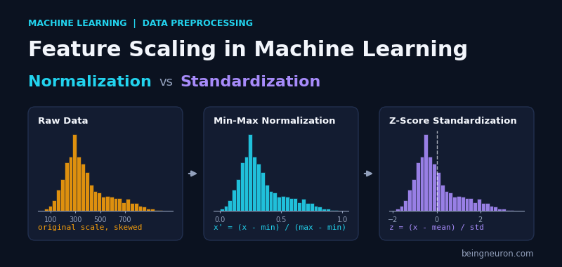
Feature scaling is the process of transforming numeric features so they share a similar range or distribution. It is one of the most common preprocessing steps in machine learning, and skipping it can quietly cut a model’s accuracy by 20 to 30 percentage points. In the experiment later in this article, a K-Nearest Neighbors classifier on the Wine dataset scores 69.1% with raw features and 94.9% after scaling, with no other change.

This guide explains what feature scaling is, why many algorithms need it, how normalization and standardization differ, and how to choose between them. You will also build a complete scikit-learn workflow, avoid the data leakage mistake that affects many beginner projects, and learn which models can safely ignore scaling.

What Is Feature Scaling?

A feature is one input column in your dataset, such as age, income, or blood pressure. Different features are measured in different units, so their numbers live on very different scales. Age ranges from 0 to 100. Annual income ranges from 0 to 1,000,000. Feature scaling rewrites these columns so that no feature dominates simply because its numbers are larger.

Scaling changes the units of a feature but not the information it carries. The order of the values and the relative gaps between them are preserved. A person who is the tallest in the dataset is still the tallest after scaling.

Why Scale Features? A Concrete Example

The scikit-learn Wine dataset describes 178 wines using 13 chemical measurements. Two of them are alcohol (about 11 to 15 percent) and proline (about 278 to 1,680 mg/L). Proline is hundreds of times larger numerically.

Horizontal range bars on one 0 to 1700 axis: alcohol from 11.0 to 14.8, proline from 278 to 1680.Same axis, very different ranges (Wine dataset)Alcohol (%)11.0 to 14.8: a thin sliverProline (mg/L)278 to 1,680050010001500Raw feature value

Many algorithms compare examples using distance or update weights using gradients. Both react strongly to feature magnitude:

• Distance-based models (KNN, K-Means, SVM with an RBF kernel) add squared differences across features. A feature with a larger range contributes more to that sum, so it controls which points count as “close”.
• Gradient-based models (linear and logistic regression, neural networks) train faster and more stably when features share a similar scale, because the loss surface is rounder and gradient descent can use a larger learning rate.
• Regularized models (Ridge, Lasso, Elastic Net) penalize coefficient size. A feature measured in tiny units needs a huge coefficient, which the penalty then unfairly shrinks.
• PCA looks for directions of maximum variance. Unscaled data makes the largest-unit feature dominate the first component.

Which Algorithms Need Feature Scaling?

Algorithm family	Needs scaling?	Reason
KNN, K-Means, DBSCAN	Yes	Based on distances between points
SVM (especially RBF kernel)	Yes	Kernels use distances; margin depends on feature scale
Linear / Logistic Regression with regularization	Yes	Penalty depends on coefficient size
Neural networks	Yes	Faster, more stable gradient descent
PCA, LDA	Yes	Variance-based; large units dominate
Decision trees, Random Forest, Gradient Boosting	No	Splits depend on value order, not magnitude
Naive Bayes	Usually no	Models each feature independently

Normalization (Min-Max Scaling)

Normalization, in the most common sense, rescales a feature to a fixed range, usually 0 to 1. It is also called Min-Max scaling.

x_scaled = (x − x_min) / (x_max − x_min)

• x is the original value of the feature for one example.
• x_min is the smallest value of that feature in the training data.
• x_max is the largest value of that feature in the training data.
• x_scaled is the new value, between 0 and 1 for training data.

Worked example. Take five heights in centimeters: 150, 160, 170, 180, 190. Here x_min = 150 and x_max = 190, so the range is 40. The height 170 becomes (170 − 150) / 40 = 0.5. The five values become 0, 0.25, 0.5, 0.75, and 1.

To use a different range [a, b], multiply the result by (b − a) and add a. In scikit-learn this is the feature_range parameter.

Strengths: bounded output, simple to interpret, works well for image pixels (0 to 255 becomes 0 to 1) and neural network inputs. Weakness: the minimum and maximum come from only two data points, so a single outlier can compress every other value into a narrow band (see the outlier section below).

Standardization (Z-Score Scaling)

Standardization recenters a feature to have a mean of 0 and a standard deviation of 1.

z = (x − μ) / σ

• x is the original value.
• μ (mu) is the mean of that feature in the training data.
• σ (sigma) is the standard deviation of that feature in the training data: the typical distance of a value from the mean.
• z is the standardized value, also called the z-score. It tells you how many standard deviations the value lies above or below the mean.

Worked example. For the same heights, μ = 170 and σ = 14.14 (population standard deviation, which is what scikit-learn uses). The height 190 gives z = (190 − 170) / 14.14 = 1.41. The five values become −1.41, −0.71, 0, 0.71, and 1.41.

Standardized values are not bounded. A value three standard deviations above the mean becomes 3. Standardization does not make data normally distributed: if a feature is skewed before standardizing, it is equally skewed afterward.

Heights 150 to 190 cm as raw values, Min-Max scaled to 0 to 1, and standardized to z-scores.Scaling changes the axis, not the patternRaw height (cm)150160170180190Min-Max scaled (range 0 to 1)00.250.50.751Standardized (mean 0, std 1)-1.41-0.7100.711.41

Normalization vs Standardization: Key Differences

Aspect	Normalization (Min-Max)	Standardization (Z-score)
Formula	(x − min) / (max − min)	(x − mean) / std
Output range	Fixed, usually [0, 1]	Unbounded, centered at 0
Sensitivity to outliers	High (min and max set the scale)	Moderate (mean and std are affected, but less)
Changes the shape of the distribution	No	No
Good default for	Images, bounded inputs, neural networks, features with known limits	Linear models, SVM, PCA, features that look roughly bell-shaped
scikit-learn class	MinMaxScaler	StandardScaler

How to Choose

1. Start with standardization for SVM, logistic regression, linear regression with regularization, and PCA. It is the safest general default.
2. Use Min-Max scaling when you need values inside a fixed range (pixel intensities, inputs to a sigmoid layer) or when the feature has natural hard limits and no strong outliers.
3. Use robust scaling when the data has outliers you cannot remove.
4. When unsure, test both with cross-validation. The difference is often small, as the experiment below shows.

How Outliers Affect Each Method

Suppose a feature holds the values 10, 12, 14, 16, 18, and 100. The value 100 is an outlier.

• Min-Max: min = 10 and max = 100, so the five normal values map to 0, 0.022, 0.044, 0.067, and 0.089. They are squeezed into 9% of the range.
• Standardization: the mean is 28.3 and the standard deviation is 32.2. The five normal values map to about −0.57, −0.51, −0.45, −0.38, and −0.32. They are still squeezed together, and the outlier sits at 2.23.
• Robust scaling: uses the median (15) and the interquartile range (IQR = 5). The normal values map to −1, −0.6, −0.2, 0.2, and 0.6. The outlier becomes 17, far from the rest, but it no longer distorts the scale of the normal points.

The values 10, 12, 14, 16, 18 and 100 after Min-Max, standard and robust scaling.One outlier (100) and five normal valuesMin-Max: normal values span only 0 to 0.0901 (outlier)Standardized: normal values span only 0.25 z-units-0.572.23 (outlier)Robust: normal values span 1.6 units, outlier stays at 17-117 (outlier)

Other Scalers Worth Knowing

• RobustScaler: subtracts the median and divides by the IQR (the distance between the 25th and 75th percentiles). Best for outlier-heavy data.
• MaxAbsScaler: divides each feature by its maximum absolute value, giving a range of [−1, 1] without shifting the data. It keeps zeros as zeros, so it suits sparse matrices such as TF-IDF.
• Normalizer: a different operation despite the similar name. It rescales each row (each sample) to unit length. It is useful for text and for cosine similarity, not for balancing columns.
• PowerTransformer / log transform: reduce skewness. They change the distribution shape, which pure scaling does not. Heavily right-skewed features such as income often benefit from a log transform first, then standardization.

Scaling Changes Who Your Nearest Neighbor Is

Here is a small calculation that shows why unscaled distances mislead. Using the Wine dataset’s alcohol and proline features, consider a reference wine P and two candidates:

• P = (alcohol 13.5, proline 1000)
• Q = (alcohol 12.2, proline 1020)
• R = (alcohol 13.4, proline 1300)

Q is chemically different from P in alcohol (a gap of 1.3 points, which is more than one standard deviation), while R matches P in alcohol but has a much higher proline. The Euclidean distance is sqrt((a₁ − a₂)² + (p₁ − p₂)²), where a is alcohol and p is proline.

Raw distances: P to Q 20.0, P to R 300.0. Standardized distances: P to Q 1.63, P to R 0.99.Distance from P to each candidateRaw featuresStandardized featuresP to Q20.0 (nearest)P to R300.0P to Q1.63P to R0.99 (nearest)Proline dominates: Q winsBoth features count: R winsScaled with std of 0.8 for alcohol and 304 for proline (training-set values from the Wine data)

With raw values, the distance P to Q is about 20.0 and P to R is 300.0, so a KNN model picks Q. After standardization (alcohol std 0.8, proline std 304), P to Q is about 1.63 and P to R is 0.99, so the model picks R. The prediction changes because the geometry changed. Which answer is “right” depends on whether alcohol and proline should matter equally; scaling makes that assumption explicit instead of letting the units decide.

Feature Scaling in Python with Scikit-Learn

This tutorial uses the Wine dataset (178 samples, 13 numeric features, 3 wine classes). The task is to predict the grape variety from chemical measurements.

Step 1: Load the data and inspect the scales

import numpy as np
from sklearn.datasets import load_wine
from sklearn.model_selection import train_test_split

X, y = load_wine(return_X_y=True)

X_train, X_test, y_train, y_test = train_test_split(
    X, y, test_size=0.25, random_state=42, stratify=y
)

# Columns 0 = alcohol, 12 = proline
print("Mean:", np.round(X_train[:, [0, 12]].mean(axis=0), 2))
print("Std: ", np.round(X_train[:, [0, 12]].std(axis=0), 2))

Output:

Mean: [ 12.97 747.41]
Std:  [  0.8  303.76]

train_test_split divides the data into a training set (75%) and a test set (25%). stratify=y keeps the class proportions equal in both sets. random_state=42 makes the split repeatable. The output confirms the problem: proline has a standard deviation roughly 380 times larger than alcohol.

Step 2: Train a baseline model without scaling

from sklearn.neighbors import KNeighborsClassifier

knn = KNeighborsClassifier()           # default: 5 neighbors
knn.fit(X_train, y_train)
print("Raw accuracy:", round(knn.score(X_test, y_test), 3))

Output:

Raw accuracy: 0.778

Step 3: Apply standardization and normalization

from sklearn.preprocessing import StandardScaler, MinMaxScaler

# Standardization
std_scaler = StandardScaler()
X_train_std = std_scaler.fit_transform(X_train)   # learn mean/std, then transform
X_test_std  = std_scaler.transform(X_test)        # reuse training mean/std

# Normalization (Min-Max)
mm_scaler = MinMaxScaler()
X_train_mm = mm_scaler.fit_transform(X_train)
X_test_mm  = mm_scaler.transform(X_test)

for name, (tr, te) in {"Standardized": (X_train_std, X_test_std),
                       "Min-Max": (X_train_mm, X_test_mm)}.items():
    model = KNeighborsClassifier().fit(tr, y_train)
    print(f"{name} accuracy:", round(model.score(te, y_test), 3))

Output:

Standardized accuracy: 0.933
Min-Max accuracy: 0.978

Key functions: fit() computes the statistics (mean and standard deviation, or minimum and maximum) from the data you pass. transform() applies those stored statistics. fit_transform() does both in one call, and you should call it on training data only.

Accuracy jumps from 77.8% to 93.3% and 97.8%. The 4.5-point gap between the two scalers equals two test samples out of 45, so it is noise rather than a real difference. A more reliable comparison needs cross-validation.

Step 4: Compare scalers with cross-validation and pipelines

from sklearn.pipeline import make_pipeline
from sklearn.model_selection import cross_val_score
from sklearn.svm import SVC

models = {
    "KNN, raw":          KNeighborsClassifier(),
    "KNN, standardized": make_pipeline(StandardScaler(), KNeighborsClassifier()),
    "KNN, min-max":      make_pipeline(MinMaxScaler(), KNeighborsClassifier()),
    "SVM, raw":          SVC(),
    "SVM, standardized": make_pipeline(StandardScaler(), SVC()),
}

for name, model in models.items():
    scores = cross_val_score(model, X, y, cv=5)
    print(f"{name:20s} {scores.mean():.3f}")

Output:

KNN, raw             0.691
KNN, standardized    0.949
KNN, min-max         0.950
SVM, raw             0.663
SVM, standardized    0.983

Wine dataset accuracy: KNN raw 0.691, KNN standardized 0.949, KNN min-max 0.950, SVM raw 0.663, SVM standardized 0.983.5-fold CV accuracy on the Wine dataset0.00.250.50.751.00.6910.9490.9500.6630.983KNN rawKNN standardizedKNN min-maxSVM rawSVM standardizedRed bars: no scaling

make_pipeline chains the scaler and the model into one object. During cross-validation, the pipeline refits the scaler inside every fold using only that fold’s training portion. This is the correct way to avoid data leakage, covered next.

Data Leakage: The Most Common Scaling Mistake

Data leakage happens when information from the test set influences training. If you compute the mean and standard deviation on the full dataset before splitting, the test data has already shaped the scaler. Your test score becomes slightly optimistic and no longer reflects how the model behaves on truly new data.

Wrong order scales before splitting. Correct order splits first, fits the scaler on training data, and applies it to the test data.Wrong: scaler sees the test dataAll datafit_transform onALL dataSplit train / testRight: scaler learns from training data onlySplit firstfit on train(mean, std)transform trainand testTrain modelA Pipeline performs the right-hand workflow automatically, including inside cross-validation.

# Wrong
X_scaled = StandardScaler().fit_transform(X)
X_train, X_test, y_train, y_test = train_test_split(X_scaled, y)

# Right
X_train, X_test, y_train, y_test = train_test_split(X, y)
scaler = StandardScaler().fit(X_train)
X_train, X_test = scaler.transform(X_train), scaler.transform(X_test)

The same rule applies when you receive new data in production: use the scaler saved from training (for example, with joblib.dump), never refit it on incoming data.

Common Mistakes and How to Fix Them

Fitting the scaler on the test set

Calling fit_transform on X_test gives the test set its own mean and standard deviation, so train and test are on different scales. Fix: call transform on the test set.

Scaling the target variable by accident

For classification, never scale y. For regression, scaling y is optional and rarely needed for tree models; if you do it, remember to invert predictions with inverse_transform.

Scaling one-hot encoded or binary columns

Columns that already contain 0 and 1 do not need standardization, and it makes them harder to interpret. Use ColumnTransformer to scale only the numeric columns.

from sklearn.compose import ColumnTransformer
from sklearn.preprocessing import OneHotEncoder

preprocess = ColumnTransformer([
    ("num", StandardScaler(), ["age", "income"]),
    ("cat", OneHotEncoder(handle_unknown="ignore"), ["city"]),
])

ValueError: Expected 2D array, got 1D array instead

Scalers expect a table with rows and columns. A single column must be reshaped: scaler.fit_transform(x.reshape(-1, 1)), or select it with double brackets, df[["age"]].

ValueError: could not convert string to float

The scaler received text columns. Encode categories first or use a ColumnTransformer to pass only numeric columns.

NotFittedError: This StandardScaler instance is not fitted yet

You called transform before fit. Call fit (or fit_transform) on training data first.

Scaling tree-based models unnecessarily

It does no harm, but it adds code and makes feature importances harder to read in original units. Skip it for Random Forest and Gradient Boosting.

Ignoring outliers and skew

Check histograms or df.describe() before choosing a scaler. If a feature is heavily skewed, apply a log or power transform, then scale.

Real-World Applications

• Medical diagnosis: blood pressure, cholesterol, and age sit on very different scales. Standardization lets a logistic regression or SVM weigh them fairly.
• Credit scoring: income can be a thousand times larger than the number of late payments. Scaling prevents income from dominating regularized models.
• Image classification: pixel values from 0 to 255 are divided by 255, a Min-Max scaling that stabilizes neural network training.
• Customer segmentation: K-Means on age, spend, and visit frequency produces meaningless clusters without scaling because spend dominates the distance.
• Recommendation systems: similarity between users depends on rating scales and activity counts that must be put on a common footing.

Advantages and Limitations of Feature Scaling

Advantages

• Improves accuracy of distance-based and margin-based models.
• Speeds up gradient descent convergence.
• Makes regularization treat every feature fairly.
• Makes coefficients and distances comparable across features.

Limitations

• Does not fix skewed distributions or outliers by itself.
• Scaled values lose their original units, which complicates interpretation unless you invert the transform.
• Requires storing the fitted scaler for use in production.
• Adds no benefit to tree-based models.

Best Practices Checklist

1. Split the data before fitting any scaler.
2. Wrap the scaler and model in a Pipeline.
3. Pick the scaler from the model type and the data (outliers, bounds, skew).
4. Compare options with cross-validation, not a single split.
5. Save the fitted scaler together with the model.
6. Scale only numeric features that need it.

Related reading on BeingNeuron: K-Nearest Neighbors (KNN) Algorithm Explained, Support Vector Machines (SVM): How They Work, and Cross-Validation in Machine Learning: K-Fold Explained.

Frequently Asked Questions

What is the difference between normalization and standardization?

Normalization (Min-Max scaling) squeezes values into a fixed range such as 0 to 1 using the minimum and maximum. Standardization shifts values to a mean of 0 and a standard deviation of 1 using the mean and standard deviation. The first gives bounded output; the second does not.

Which is better, normalization or standardization?

Neither is better in every case. Standardization is the safer default for SVM, linear models, and PCA. Min-Max suits bounded inputs like images and neural networks. In the Wine experiment above, both gave the same cross-validated KNN accuracy (about 95%).

Do I need to scale features for decision trees and random forests?

No. Trees split on thresholds, so only the order of the values matters. Monotonic transformations like scaling leave the splits unchanged.

Should I scale before or after train-test split?

After. Split first, fit the scaler on the training set only, then transform both sets. Fitting before the split leaks test information into training.

Does standardization make data normally distributed?

No. It changes the mean and spread but keeps the shape. A skewed feature stays skewed. Use a log or PowerTransformer to reduce skew.

Should I scale the target variable?

Never for classification. For regression it is usually unnecessary, though it can help neural networks. If you scale it, invert the predictions before reporting errors.

How do I handle outliers when scaling?

Use RobustScaler, clip extreme values, or apply a log transform first. Avoid Min-Max scaling when large outliers are present.

Can I scale categorical variables?

No. Encode them first (for example with one-hot encoding), then scale only genuine numeric columns.

What is the difference between StandardScaler and Normalizer in scikit-learn?

StandardScaler works on columns (features). Normalizer works on rows (samples), rescaling each one to unit length. They solve different problems.

Conclusion

Feature scaling does not add information to your data, but it changes which patterns a model can see. In the Wine experiment, the same KNN model moved from 69% to 95% accuracy once alcohol and proline were measured on comparable scales. The rules are short: scale for distance-based, margin-based, regularized, and gradient-trained models; skip it for trees; choose standardization by default and Min-Max for bounded inputs; handle outliers with robust scaling; and always fit the scaler on training data inside a pipeline.

Next, put scaling to work in a real model by reading about the K-Nearest Neighbors algorithm, where it matters most.