
Avl Tree Visualization
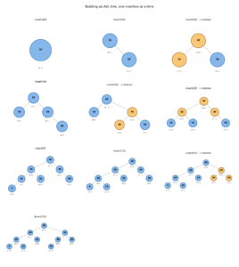
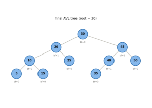
An AVL Tree is a special type of Binary Search Tree that automatically keeps itself balanced.
A normal Binary Search Tree can provide very fast searching, insertion, and deletion when the tree remains balanced. In that situation, these operations can take O(log n) time.
However, a normal Binary Search Tree does not automatically control its shape. If we insert values in a certain order, the tree can become very tall. When that happens, the tree can start behaving like a linked list, and searching can take O(n) time.
An AVL Tree solves this problem by checking its balance after every insertion and deletion. When the tree becomes unbalanced, it changes its structure using rotations.
In this article, we will learn how AVL Trees work, why we need them, how to calculate their balance factor, how rotations work, and how to implement an AVL Tree in C++.
What Is a Binary Search Tree?
Before understanding an AVL Tree, we need to understand a Binary Search Tree.
A Binary Search Tree, usually called a BST, stores values according to a simple rule.
Every value in the left subtree must be smaller than the current node.
Every value in the right subtree must be larger than the current node.
For example:
        50
       /  \
     30    70
    /  \   / \
   20  40 60 80
The root contains 50.
Values smaller than 50 go to the left.
Values larger than 50 go to the right.
The same rule continues inside every subtree.
For example, 30 has 20 on its left because 20 is smaller than 30. It has 40 on its right because 40 is larger than 30.
This structure allows us to search efficiently.
Suppose we want to find 60.
We start at 50.
Since 60 is greater than 50, we move to the right.
We reach 70.
Since 60 is smaller than 70, we move to the left.
We reach 60.
We found the value after checking only a few nodes.
The Problem With a Normal Binary Search Tree
A Binary Search Tree does not automatically balance itself.
Suppose we insert these values in this order:
10
20
30
40
50
The tree can become:
10
  \
   20
     \
      30
        \
         40
           \
            50
This tree still follows all the rules of a Binary Search Tree.
However, the structure is inefficient.
The tree has almost become a linked list.
If we search for 50, we have to visit:
10 → 20 → 30 → 40 → 50
If the tree contains one million nodes and has this shape, a search could require almost one million comparisons.
The search time becomes O(n).
A balanced tree gives us a much smaller height.
For one million nodes, a balanced tree can have a height close to log₂(1,000,000), which is about 20.
This means we can search through a very large collection while checking only a small number of levels.
What Is an AVL Tree?
An AVL Tree keeps the Binary Search Tree rules while also keeping the tree balanced.
AVL stands for Adelson Velsky and Landis, the names of the researchers who introduced this data structure.
The main rule is simple.
For every node, the height difference between the left subtree and the right subtree must not be greater than 1.
The tree checks this difference using something called the balance factor.
If the tree becomes unbalanced, the AVL Tree performs a rotation to fix its structure.
The AVL Tree therefore combines two important ideas:
Binary Search Tree
+
Automatic balancing
=
AVL Tree
What Is Height?
Height tells us how many levels exist below a node.
For our implementation, we use the following definition:
Empty tree = 0
New node = 1
For example:
        50
       /  \
     30    70
The nodes 30 and 70 have height 1.
The node 50 has height 2.
Now consider:
        50
       /
     30
    /
   20
The node 20 has height 1.
The node 30 has height 2.
The node 50 has height 3.
We calculate the height of a node using:
height = 1 + maximum(left height, right height)
The 1 represents the current node.
What Is the Balance Factor?
The balance factor tells us whether a node has a balanced structure.
We calculate it using:
Balance Factor =
Height of Left Subtree − Height of Right Subtree
Suppose a node has:
Left height = 3
Right height = 2
Then:
Balance Factor = 3 − 2
               = 1
The node is balanced.
Now suppose we have:
Left height = 3
Right height = 1
Then:
Balance Factor = 3 − 1
               = 2
The node is now unbalanced.
An AVL Tree allows these balance factors:
−1
 0
+1
When the balance factor becomes:
−2
or:
+2
the node needs rebalancing.
Why Does an AVL Tree Need Rotations?
When we insert a new value, we can make one side of the tree taller than the other side.
For example:
      30
     /
   20
  /
10
The left side has become much taller than the right side.
The balance factor of 30 is:
2
The tree needs to change its structure.
We call this structural change a rotation.
A rotation moves nodes around while keeping the Binary Search Tree ordering correct.
AVL Trees use four main cases:
Left Left
Right Right
Left Right
Right Left
Left Left Case
Consider inserting:
30
20
10
The tree becomes:
      30
     /
   20
  /
10
The new value moved left from 30 and then left again from 20.
This creates the Left Left case.
The balance factor of 30 becomes +2.
We fix the tree using a right rotation.
Before the rotation:
      30
     /
   20
  /
10
After the rotation:
     20
    /  \
  10    30
The tree becomes balanced.
Right Right Case
Now consider inserting:
10
20
30
The tree becomes:
10
  \
   20
     \
      30
The new value moved right from 10 and then right again from 20.
This creates the Right Right case.
The balance factor of 10 becomes −2.
We fix it using a left rotation.
Before the rotation:
10
  \
   20
     \
      30
After the rotation:
     20
    /  \
  10    30
The tree becomes balanced.
Left Right Case
Consider inserting:
30
10
20
The tree becomes:
      30
     /
   10
     \
      20
The new value moved left from 30 and then right from 10.
This creates the Left Right case.
We need two rotations.
First, we perform a left rotation on 10.
      30
     /
   20
  /
10
Now the tree has become a Left Left case.
We perform a right rotation on 30.
The final tree becomes:
     20
    /  \
  10    30
Right Left Case
Now consider inserting:
10
30
20
The tree becomes:
10
  \
   30
   /
  20
The new value moved right from 10 and then left from 30.
This creates the Right Left case.
We also need two rotations.
First, we perform a right rotation on 30.
10
  \
   20
     \
      30
Now the tree has become a Right Right case.
We perform a left rotation on 10.
The final tree becomes:
     20
    /  \
  10    30
Rotation Rules
We can summarize the four cases like this:
| Case | First Rotation | Second Rotation |
|---|---|---|
| Left Left | Right rotation | None |
| Right Right | Left rotation | None |
| Left Right | Left rotation | Right rotation |
| Right Left | Right rotation | Left rotation |
Once you understand these four cases, the AVL insertion algorithm becomes much easier to follow.
Creating an AVL Tree Node in C++
Now let’s start implementing an AVL Tree.
#include <iostream>
#include <algorithm>

using namespace std;

struct Node {
    int key;
    Node* left;
    Node* right;
    int height;

    Node(int value) {
        key = value;
        left = nullptr;
        right = nullptr;
        height = 1;
    }
};
The Node structure represents one node in our tree.
Each node contains four important pieces of information.
int key;
This stores the value.
For example, if we insert 50, the key becomes 50.
Next:
Node* left;
This pointer stores the address of the left child.
Then:
Node* right;
This pointer stores the address of the right child.
Finally:
int height;
This stores the height of the node.
The constructor creates a new node:
Node(int value) {
    key = value;
    left = nullptr;
    right = nullptr;
    height = 1;
}
When we create a new node, it does not have any children.
Therefore, we set both child pointers to nullptr.
We also give the new node a height of 1.
Getting the Height
Now we need a function that returns the height of a node.
int getHeight(Node* node) {

    if (node == nullptr)
        return 0;

    return node->height;
}
The first condition checks whether the node exists.
if (node == nullptr)
    return 0;
If the node does not exist, we return 0.
Otherwise, we return the height stored inside the node:
return node->height;
This function makes the rest of the AVL code easier to read.
Calculating the Balance Factor
Next, we create a function that calculates the balance factor.
int getBalance(Node* node) {

    if (node == nullptr)
        return 0;

    return getHeight(node->left)
         - getHeight(node->right);
}
The function first checks whether the node exists.
Then it gets the height of the left subtree:
getHeight(node->left)
It also gets the height of the right subtree:
getHeight(node->right)
Finally, it subtracts the right height from the left height.
left height − right height
For example:
Left height = 3
Right height = 1

Balance Factor = 3 − 1
               = 2
The node needs rebalancing.
Right Rotation
Now we can implement the right rotation.
Node* rightRotate(Node* y) {

    Node* x = y->left;
    Node* T2 = x->right;

    x->right = y;
    y->left = T2;

    y->height = 1 + max(
        getHeight(y->left),
        getHeight(y->right)
    );

    x->height = 1 + max(
        getHeight(x->left),
        getHeight(x->right)
    );

    return x;
}
This code can look confusing at first, so let’s understand it carefully.
Imagine that we have:
      y
     /
    x
   / \
  A   B
We want to move x upward.
First:
Node* x = y->left;
We store the left child of y inside x.
Then:
Node* T2 = x->right;
We temporarily save the right subtree of x.
This is important because we do not want to lose those nodes.
Now:
x->right = y;
We make y the right child of x.
Then:
y->left = T2;
We attach the saved subtree to y.
The structure changes from:
      y
     /
    x
   / \
  A   B
to:
    x
   / \
  A   y
     /
    B
The tree remains a valid Binary Search Tree.
Updating Heights After a Rotation
The rotation changes the positions of the nodes.
Therefore, their heights can also change.
We update the height of y:
y->height = 1 + max(
    getHeight(y->left),
    getHeight(y->right)
);
Then we update the height of x:
x->height = 1 + max(
    getHeight(x->left),
    getHeight(x->right)
);
Finally, we return x:
return x;
We return x because it has become the new root of this part of the tree.
Left Rotation
Now let’s implement a left rotation.
Node* leftRotate(Node* x) {

    Node* y = x->right;
    Node* T2 = y->left;

    y->left = x;
    x->right = T2;

    x->height = 1 + max(
        getHeight(x->left),
        getHeight(x->right)
    );

    y->height = 1 + max(
        getHeight(y->left),
        getHeight(y->right)
    );

    return y;
}
This operation performs the opposite movement.
Suppose we have:
x
 \
  y
 / \
A   B
The rotation moves y upward:
    y
   / \
  x   B
 / \
A   T2
We save the middle subtree first:
Node* T2 = y->left;
Then we move x below y:
y->left = x;
Finally, we attach the saved subtree to x:
x->right = T2;
We then update the heights.
Inserting a Value Into an AVL Tree
Now we can implement insertion.
Node* insert(Node* node, int key) {

    if (node == nullptr)
        return new Node(key);

    if (key < node->key)
        node->left = insert(node->left, key);

    else if (key > node->key)
        node->right = insert(node->right, key);

    else
        return node;

    node->height = 1 + max(
        getHeight(node->left),
        getHeight(node->right)
    );

    int balance = getBalance(node);

    if (balance > 1 &&
        key < node->left->key)
        return rightRotate(node);

    if (balance < -1 &&
        key > node->right->key)
        return leftRotate(node);

    if (balance > 1 &&
        key > node->left->key) {

        node->left =
            leftRotate(node->left);

        return rightRotate(node);
    }

    if (balance < -1 &&
        key < node->right->key) {

        node->right =
            rightRotate(node->right);

        return leftRotate(node);
    }

    return node;
}
This function performs several important tasks.
Step 1: Find the Correct Position
We first check whether the current node is empty.
if (node == nullptr)
    return new Node(key);
If the current position is empty, we create the new node.
Next, we compare the new value with the current node.
if (key < node->key)
    node->left = insert(node->left, key);
If the new value is smaller, we move to the left.
If the new value is larger:
else if (key > node->key)
    node->right = insert(node->right, key);
we move to the right.
This part works like normal Binary Search Tree insertion.
Step 2: Handle Duplicate Values
If the new value equals the current value, this implementation does nothing.
else
    return node;
Therefore, our AVL Tree does not store duplicate values.
You can change this behavior if your application needs duplicate values.
Step 3: Update the Height
After insertion, we update the height:
node->height = 1 + max(
    getHeight(node->left),
    getHeight(node->right)
);
The recursive function returns through the tree.
Each ancestor updates its height as the function moves upward.
Step 4: Calculate the Balance Factor
Next:
int balance = getBalance(node);
We calculate the balance factor.
If the value is:
−1
0
+1
the node remains balanced.
If the value becomes:
−2
+2
we need to perform a rotation.
Detecting the Left Left Case
The following code checks for the Left Left case:
if (balance > 1 &&
    key < node->left->key)
    return rightRotate(node);
The balance is greater than 1, which means the left side has become too tall.
The inserted value is smaller than the left child.
Therefore, the value entered through the left side and then the left side again.
We perform a right rotation.
Detecting the Right Right Case
The following code checks for the Right Right case:
if (balance < -1 &&
    key > node->right->key)
    return leftRotate(node);
The balance is less than −1, which means the right side has become too tall.
The inserted value is larger than the right child.
Therefore, the value entered through the right side and then the right side again.
We perform a left rotation.
Detecting the Left Right Case
The following code handles the Left Right case:
if (balance > 1 &&
    key > node->left->key) {

    node->left =
        leftRotate(node->left);

    return rightRotate(node);
}
We need two rotations.
First, we rotate the left child to the left:
node->left =
    leftRotate(node->left);
Then we rotate the current node to the right:
return rightRotate(node);
This converts the Left Right shape into a balanced structure.
Detecting the Right Left Case
The following code handles the Right Left case:
if (balance < -1 &&
    key < node->right->key) {

    node->right =
        rightRotate(node->right);

    return leftRotate(node);
}
First, we rotate the right child to the right.
Then we rotate the current node to the left.
This produces a balanced tree.
Why Does the Insert Function Return a Node?
You may wonder why we write:
root = insert(root, 30);
instead of simply:
insert(root, 30);
The reason is that a rotation can change the root of a subtree.
For example, before a rotation:
      30
     /
   20
  /
10
After a right rotation:
     20
    /  \
  10    30
The root changed from 30 to 20.
The function must return the new root.
That is why we write:
root = insert(root, 30);
We store the returned node as the new root.
Inorder Traversal
Let’s create an inorder traversal function.
void inorder(Node* root) {

    if (root == nullptr)
        return;

    inorder(root->left);

    cout << root->key << " ";

    inorder(root->right);
}
The function visits the nodes in this order:
Left
Root
Right
An inorder traversal of a Binary Search Tree produces values in sorted order.
For example:
        20
       /  \
     10    30
The traversal visits:
10
20
30
Therefore, the output becomes:
10 20 30
Complete AVL Tree Program
Here is the complete AVL Tree implementation:
#include <iostream>
#include <algorithm>

using namespace std;

struct Node {

    int key;

    Node* left;
    Node* right;

    int height;

    Node(int value) {

        key = value;

        left = nullptr;
        right = nullptr;

        height = 1;
    }
};

int getHeight(Node* node) {

    if (node == nullptr)
        return 0;

    return node->height;
}

int getBalance(Node* node) {

    if (node == nullptr)
        return 0;

    return getHeight(node->left)
         - getHeight(node->right);
}

Node* rightRotate(Node* y) {

    Node* x = y->left;

    Node* T2 = x->right;

    x->right = y;

    y->left = T2;

    y->height = 1 + max(
        getHeight(y->left),
        getHeight(y->right)
    );

    x->height = 1 + max(
        getHeight(x->left),
        getHeight(x->right)
    );

    return x;
}

Node* leftRotate(Node* x) {

    Node* y = x->right;

    Node* T2 = y->left;

    y->left = x;

    x->right = T2;

    x->height = 1 + max(
        getHeight(x->left),
        getHeight(x->right)
    );

    y->height = 1 + max(
        getHeight(y->left),
        getHeight(y->right)
    );

    return y;
}

Node* insert(Node* node, int key) {

    if (node == nullptr)
        return new Node(key);

    if (key < node->key) {

        node->left =
            insert(node->left, key);
    }

    else if (key > node->key) {

        node->right =
            insert(node->right, key);
    }

    else {

        return node;
    }

    node->height = 1 + max(
        getHeight(node->left),
        getHeight(node->right)
    );

    int balance = getBalance(node);

    if (balance > 1 &&
        key < node->left->key) {

        return rightRotate(node);
    }

    if (balance < -1 &&
        key > node->right->key) {

        return leftRotate(node);
    }

    if (balance > 1 &&
        key > node->left->key) {

        node->left =
            leftRotate(node->left);

        return rightRotate(node);
    }

    if (balance < -1 &&
        key < node->right->key) {

        node->right =
            rightRotate(node->right);

        return leftRotate(node);
    }

    return node;
}

void inorder(Node* root) {

    if (root == nullptr)
        return;

    inorder(root->left);

    cout << root->key << " ";

    inorder(root->right);
}

int main() {

    Node* root = nullptr;

    root = insert(root, 30);

    root = insert(root, 20);

    root = insert(root, 10);

    root = insert(root, 25);

    root = insert(root, 28);

    root = insert(root, 40);

    root = insert(root, 50);

    cout << "Inorder traversal: ";

    inorder(root);

    cout << endl;

    return 0;
}
The program produces:
Inorder traversal: 10 20 25 28 30 40 50
The values appear in sorted order because the AVL Tree still follows all Binary Search Tree rules.
Tracing an AVL Tree Step by Step
Let’s see what happens when we insert several values.
We start with:
root = insert(root, 30);
The tree is empty, so the program creates a new node.
30
Next:
root = insert(root, 20);
Since 20 is smaller than 30, it goes to the left.
   30
  /
20
The tree remains balanced.
Now we insert:
root = insert(root, 10);
The program compares 10 with 30.
Since 10 is smaller, it moves left.
It then compares 10 with 20.
Again, 10 is smaller, so it moves left.
The tree becomes:
      30
     /
   20
  /
10
Now the balance factor of 30 becomes +2.
The program identifies the Left Left case.
It performs a right rotation.
The tree becomes:
     20
    /  \
  10    30
The AVL Tree has automatically fixed the imbalance.
Inserting 25
Now we insert 25.
     20
    /  \
  10    30
       /
      25
The tree remains balanced.
No rotation is required.
Inserting 28
Now we insert 28.
The program first compares it with 20.
Since 28 is larger, it moves right.
It compares 28 with 30.
Since 28 is smaller, it moves left.
It compares 28 with 25.
Since 28 is larger, it moves right.
The tree becomes:
     20
    /  \
  10    30
       /
      25
        \
         28
The subtree rooted at 30 now has a Left Right shape.
The AVL Tree performs two rotations.
First, it rotates 25 to the left.
Then, it rotates 30 to the right.
The subtree becomes:
      28
     /  \
   25    30
The complete tree becomes:
       20
      /  \
    10    28
         /  \
       25    30
The tree remains balanced.
Why Rotations Do Not Break the Binary Search Tree
Rotations may seem strange at first because they change the positions of nodes.
However, they do not break the Binary Search Tree rules.
Consider:
      30
     /
   20
  /  \
10    25
After a right rotation:
       20
      /  \
    10    30
         /
        25
Look at the values.
10 remains smaller than 20.
25 remains larger than 20 and smaller than 30.
30 remains larger than 20.
The structure changed, but the ordering remained correct.
That is why AVL Trees can safely use rotations.
Searching in an AVL Tree
An AVL Tree uses the same search process as a normal Binary Search Tree.
Consider:
       30
      /  \
    20    40
   /  \
 10    25
Suppose we want to find 25.
We start at 30.
Since:
25 < 30
we move left.
We reach 20.
Since:
25 > 20
we move right.
We reach 25.
We found the value.
Because the AVL Tree keeps its height small, search takes O(log n) time.
Deleting From an AVL Tree
Deletion can also make an AVL Tree unbalanced.
When we remove a node, the height of one subtree can decrease.
That change can affect the balance of its parent and other ancestors.
Therefore, an AVL Tree must check the balance after deletion as well.
The deletion process follows the normal Binary Search Tree deletion process first.
After deleting the value, the program updates the heights of the affected nodes.
Then it calculates the balance factor.
If a node becomes unbalanced, the program performs the required rotation.
The general process looks like this:
Delete the value
       ↓
Update heights
       ↓
Calculate balance factor
       ↓
Check for imbalance
       ↓
Perform rotation if necessary
       ↓
Return the new subtree root
Deletion requires more code than insertion because a Binary Search Tree has several deletion situations.
However, the balancing idea remains the same.
Time Complexity of an AVL Tree
The main advantage of an AVL Tree comes from its small height.
The standard operations have these time complexities:
| Operation | Time Complexity |
|---|---|
| Search | O(log n) |
| Insertion | O(log n) |
| Deletion | O(log n) |
| Rotation | O(1) |
| Finding minimum | O(log n) |
| Finding maximum | O(log n) |
A rotation takes O(1) time because it changes only a small number of pointers.
The tree requires O(n) memory because it stores one node for each value.
AVL Tree Compared With a Normal BST
A normal Binary Search Tree can become unbalanced.
Suppose we insert:
10
20
30
40
50
60
The tree can become:
10
  \
   20
     \
      30
        \
         40
           \
            50
              \
               60
The height becomes very large.
An AVL Tree keeps reorganizing itself.
It can produce a structure similar to:
        40
       /  \
     20    50
    /  \     \
   10   30    60
The AVL Tree keeps the height much smaller.
As a result, search remains efficient even when we insert values in sorted order.
AVL Tree Compared With a Linked List
A linked list can require O(n) time to find a value.
A badly shaped Binary Search Tree can also require O(n) time.
An AVL Tree prevents this problem by keeping its height balanced.
This allows the AVL Tree to provide O(log n) search time.
The difference becomes especially important when the tree contains a large number of nodes.
Advantages of AVL Trees
AVL Trees provide several important advantages.
Fast Searching
The tree keeps its height small, so searching normally takes O(log n) time.
Guaranteed Balance
The tree checks its balance after modifications.
This prevents the tree from becoming a long chain of nodes.
Efficient Insertion
Insertion takes O(log n) time because the tree maintains logarithmic height.
Efficient Deletion
Deletion also takes O(log n) time in the standard implementation.
Ordered Data
The tree maintains the Binary Search Tree property, so we can efficiently work with sorted data.
Disadvantages of AVL Trees
AVL Trees also have some disadvantages.
Rotations Add Complexity
A normal Binary Search Tree does not need balancing logic.
An AVL Tree needs extra code to calculate heights, calculate balance factors, and perform rotations.
Extra Memory
Each node stores a height value in addition to the key and child pointers.
More Work During Updates
The AVL Tree may perform rotations after insertion or deletion.
This gives the tree a little more work compared with an ordinary Binary Search Tree.
When Should You Use an AVL Tree?
An AVL Tree works well when an application needs ordered data and frequent searches.
It can be useful when we want predictable O(log n) performance.
AVL Trees are especially attractive when searching happens very frequently and we want the tree to remain strictly balanced.
Other balanced trees can work better for different workloads, so the best choice depends on the application.
AVL Tree vs Red Black Tree
A Red Black Tree is another popular self balancing Binary Search Tree.
Both AVL Trees and Red Black Trees provide O(log n) search, insertion, and deletion.
However, they maintain balance differently.
An AVL Tree keeps the tree more strictly balanced.
A Red Black Tree allows more flexibility in the tree structure.
Because of this difference, AVL Trees can be attractive when searching happens frequently, while Red Black Trees can work well when the application performs many insertions and deletions.
The correct choice depends on the workload.
The Complete AVL Tree Process
The easiest way to remember how an AVL Tree works is to remember the following process:
Insert a value
       ↓
Follow Binary Search Tree rules
       ↓
Update the height
       ↓
Calculate the balance factor
       ↓
Check the balance
       ↓
If balanced, keep the tree
       ↓
If unbalanced, identify the case
       ↓
Perform the required rotation
       ↓
Return the new subtree root
The same basic idea applies to deletion.
Delete a value
       ↓
Follow Binary Search Tree rules
       ↓
Update the height
       ↓
Calculate the balance factor
       ↓
Identify the imbalance
       ↓
Perform the required rotation
       ↓
Return the new subtree root
Key Points to Remember
An AVL Tree is a self balancing Binary Search Tree.
It keeps smaller values on the left and larger values on the right.
It stores the height of each node.
It calculates the balance factor using:
Height of Left Subtree − Height of Right Subtree
A balance factor of −1, 0, or +1 means the node is balanced.
A balance factor of −2 or +2 means the node needs rebalancing.
The AVL Tree uses four cases:
Left Left
Right Right
Left Right
Right Left
The Left Left case needs a right rotation.
The Right Right case needs a left rotation.
The Left Right case needs a left rotation followed by a right rotation.
The Right Left case needs a right rotation followed by a left rotation.
Because the AVL Tree keeps its height small, search, insertion, and deletion take O(log n) time.
Final Takeaway
An AVL Tree solves one of the biggest problems with a normal Binary Search Tree.
A normal Binary Search Tree can become unbalanced when we insert values in an unfortunate order.
An AVL Tree continuously monitors its balance and fixes the structure when necessary.
It uses height to measure the structure of the tree.
It uses the balance factor to detect imbalance.
It uses rotations to fix that imbalance.
The most important idea is:
Binary Search Tree
        +
Height tracking
        +
Balance factor
        +
Rotations
        =
AVL Tree
Once you understand how height, balance factor, and rotations work together, the AVL Tree implementation becomes much easier to understand.
The code may look long at first, but it mainly performs the same four tasks repeatedly:
Insert
Update height
Check balance
Rotate when necessary
That is the core idea behind an AVL Tree.