
Dijkstra’s Algorithm: How It Works, Examples, and Python Implementation
A complete guide to Dijkstra's algorithm: the relaxation step, a full worked trace, a correctness proof, tested Python code with path reconstruction, complexity for four priority queues, and why negative weights break it.
 Nov 21, 2026Published
38 min readReading time
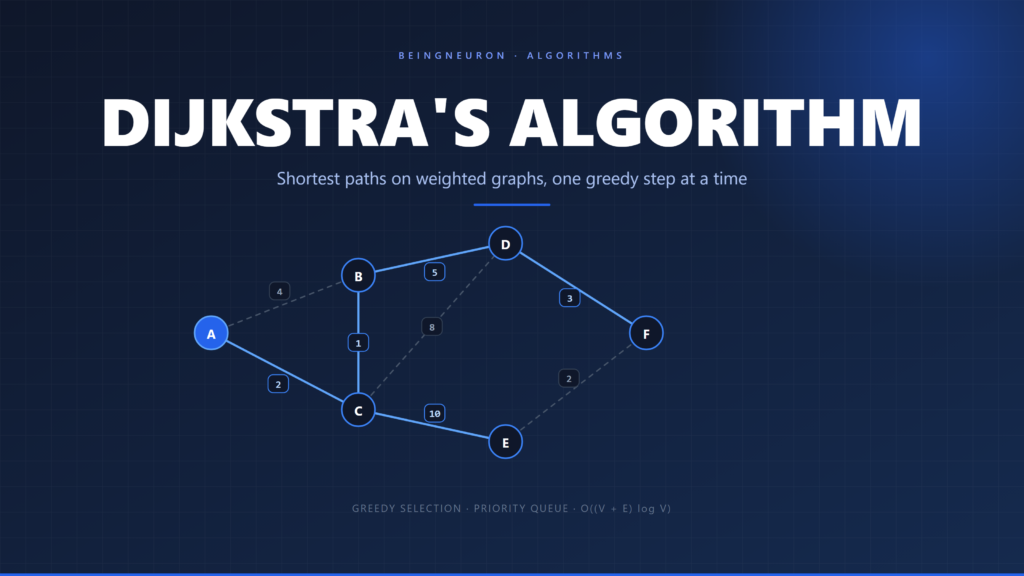
Imagine you are standing in a city you have never visited. You have a map with distances printed on every street, and you need the shortest route from your hotel to the station. You could try every possible route, but the number of routes grows explosively with the size of the map — a few dozen streets is enough to make brute force hopeless.
Dijkstra’s algorithm solves that problem in a way that feels almost too simple. It starts at your hotel, looks at the nearest street it has not yet explored, and commits to it. Then it looks at the next nearest, and commits to that. It never backtracks and never reconsiders. When it finally reaches the station, the route it has built is provably the shortest one.
That “commit and never look back” behaviour is a greedy strategy, and greedy strategies are usually wrong. Dijkstra’s genius was noticing the one condition under which this particular greedy choice is safe: every edge weight must be non-negative. Remove that condition and the algorithm does not merely get slower — it returns confidently wrong answers.
This guide covers Dijkstra’s algorithm from the ground up and then goes considerably further than most tutorials. You will see a complete trace with every queue state, a correctness proof in plain language, a tested Python implementation with path reconstruction, the real complexity of four different priority-queue choices, measured timings that contradict the usual advice about dense graphs, a step-by-step explanation of exactly why negative weights break it, and the edge cases that silently corrupt hand-written versions.
Key takeaways
- Dijkstra’s algorithm finds the shortest paths from one source vertex to every other vertex in a weighted graph.
- It grows a set of settled vertices: each step pops the unsettled vertex with the smallest tentative distance, and that distance becomes final.
- Relaxation is the only operation that ever writes a distance: if
dist[u] + w(u,v) < dist[v], thenvhas found a better route. - The greedy choice is only valid when all edge weights are non-negative. One negative edge can produce a wrong answer.
- With a binary heap the running time is O((V + E) log V); with a plain array scan on a dense graph it is O(V²).
- It answers a different question from Prim’s algorithm: shortest paths from a source, not a minimum spanning tree.
On this page
- What is Dijkstra’s algorithm?
- The problem it solves
- Core terminology
- How it works, step by step
- Relaxation: the core operation
- A complete worked example
- Why the greedy choice is safe
- Pseudocode
- Python implementation
- Reconstructing the actual path
- Time and space complexity
- Dense vs sparse graphs
- Why negative weights break it
- Dijkstra vs other algorithms
- Edge cases and common bugs
- Applications
- Variants and optimisations
- Frequently asked questions
- Practice problems
What Is Dijkstra’s Algorithm?
Dijkstra’s algorithm computes single-source shortest paths on a weighted graph whose edge weights are all zero or positive. Given a starting vertex — the source — it produces two things:
- the length of the shortest path from the source to every other vertex that can be reached;
- a parent pointer for each vertex, which together form a tree of shortest paths rooted at the source.
That second output is often skipped in tutorials, even though it is what makes the algorithm useful. A list of distances tells you a journey takes 27 minutes. The parent pointers tell you which streets to take.
Where it comes from
Edsger W. Dijkstra designed the algorithm in 1956 while working at the Mathematical Centre in Amsterdam. He was looking for something to demonstrate on the ARMAC, one of the first Dutch computers, and needed a problem that an audience could follow. He chose the shortest route between two cities on a simplified map of the Netherlands with 64 towns, and — as he later recalled — designed the method in about twenty minutes while sitting on a café terrace. He published it in 1959 in a three-page paper titled A note on two problems in connexion with graphs.
The paper is worth knowing about for a second reason: it contains the phrase that has followed the algorithm ever since. Dijkstra described his method as one that “sharpens” an upper bound on each distance until it cannot be improved, and that sharpening step is what we now call relaxation.
What it does not compute
Three distinctions cause most of the confusion around this algorithm.
| Question | Algorithm | What you get |
|---|---|---|
| Shortest path from one source to all others | Dijkstra (non-negative weights) or Bellman-Ford (any weights) | A tree of routes rooted at the source |
| Shortest path between every pair of vertices | Floyd-Warshall, or Dijkstra run once per vertex | A full distance matrix |
| Cheapest set of edges connecting all vertices | Prim’s or Kruskal’s | A minimum spanning tree, which is usually not a shortest-path tree |
The last row is the one people get wrong. A minimum spanning tree minimises the total weight of the edges used. A shortest-path tree minimises the distance from the source to each individual vertex. On the same graph the two trees can be completely different, and neither is a substitute for the other.
The Problem It Solves
Finding a shortest path by enumeration is worse than it sounds. In a graph with V vertices, the number of distinct simple paths can grow factorially, so “try them all” stops being an option long before the graph looks large. Even dynamic programming over subsets costs O(2V · V²), which is hopeless beyond roughly twenty vertices.
Dijkstra’s algorithm avoids enumeration entirely by exploiting a structural property of shortest paths: every prefix of a shortest path is itself a shortest path. If the cheapest way from the source to C passes through B, then the part of that route up to B must already be the cheapest way to reach B. If it were not, you could swap in a cheaper prefix and get a cheaper route to C, contradicting the assumption.
That single fact means distances can be built up incrementally. You never need to consider a route to a vertex before you know the best route to the vertex before it. The algorithm just has to decide the right order to grow the tree — and the right order turns out to be “cheapest first”.
Why not just use breadth-first search? BFS also explores in expanding rings, but it counts edges, not weights. On an unweighted graph the two coincide, because every edge costs the same. As soon as edges cost 1 and 100, BFS returns the route with the fewest hops, which may be the most expensive one. Dijkstra’s algorithm is, in effect, breadth-first search generalised to weighted edges — it replaces the plain queue with a priority queue.
Core Terminology
These terms appear throughout the rest of the article, and several of them are used loosely in other tutorials.
| Term | Meaning |
|---|---|
| Graph | A set of vertices joined by edges. Directed edges have a direction; undirected edges do not. |
Weight w(u,v) |
The cost of travelling from u to v. Distance, time, fuel, money — anything additive. |
| Path | A sequence of edges where each edge starts where the previous one ended. |
| Path length | The sum of the weights along the path, not the number of edges. |
| Source | The vertex the search starts from, conventionally s. |
| Shortest path | A path from the source to a target with the smallest possible total weight. |
Tentative distance dist[v] |
The best route found so far. Always the length of some real path, so it is an upper bound on the true distance. |
| Relaxation | The test that lowers a tentative distance when a better route appears. |
| Settled (or finalised, visited) | A vertex that has been popped from the priority queue. Its distance is treated as final and it is never expanded again. |
| Priority queue | A container that returns the smallest element first. Usually a binary heap. |
| Adjacency list | graph[u] holds the pairs (v, w) for every edge leaving u. The standard sparse representation. |
| Adjacency matrix | A V × V table where cell [u][v] holds the weight of the edge, or infinity when there is none. Fast lookups, quadratic memory. |
A note on “visited”. In depth-first search, “visited” means “we have been here before” and prevents infinite loops. In Dijkstra’s algorithm it means something stronger: “the shortest distance to this vertex is known and will never change”. Mixing the two meanings is the root of several bugs covered later.
How Dijkstra’s Algorithm Works, Step by Step
The algorithm maintains three pieces of state:
dist[v]— the best known distance from the source tov, initialised to infinity except for the source, which is 0.prev[v]— the vertex that offered that best distance, used to rebuild the route afterwards.- A priority queue of
(distance, vertex)pairs, containing candidates waiting to be settled.
Then it repeats one loop until the queue is empty:
- Initialise. Set
dist[source] = 0and every other distance to infinity. Clear all parent pointers. - Seed the queue. Push
(0, source). - Extract the minimum. Pop the pair with the smallest distance. If this entry is stale — its distance is larger than
dist[u]— discard it and pop again. Ifuhas already been settled, discard it too. - Settle
u. Mark it as final. Its distance will never improve, which is the claim proved in the next section. - Relax every outgoing edge. For each
(v, w)fromu, computecandidate = dist[u] + w. If it beatsdist[v], overwritedist[v], setprev[v] = u, and push(candidate, v). - Repeat from step 3.
- Stop when the queue is empty. Every reachable vertex now holds a final distance; unreachable vertices still hold infinity.
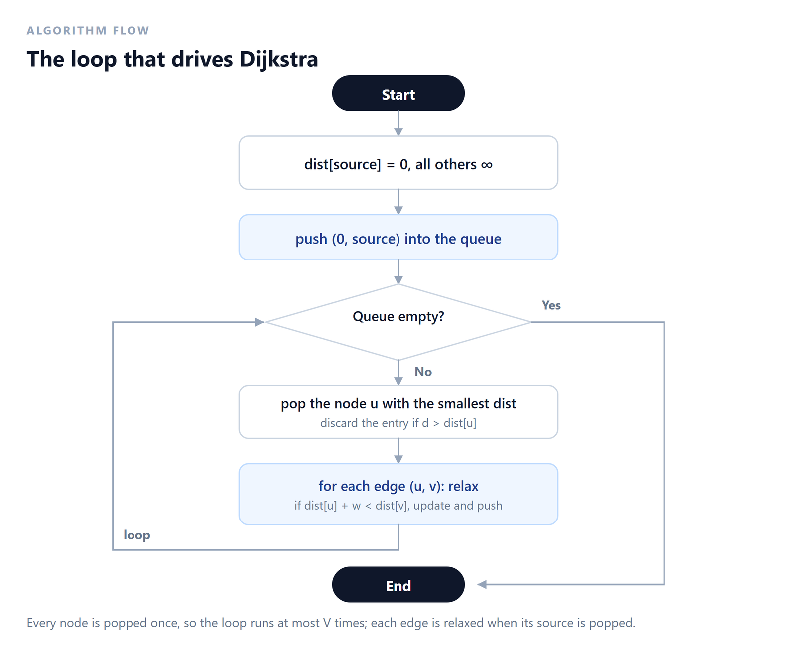
Two details in that list are easy to overlook and matter enormously in practice.
The stale-entry check is not optional. When a distance improves, a new copy is pushed and the old copy stays in the heap. Later that old copy will surface with an out-of-date value. Without the d > dist[u] guard, the algorithm would relax edges using a distance it already knows is wrong.
Settling a vertex is permanent. Once u is popped, its outgoing edges are relaxed exactly once. That is what makes the algorithm linear in the number of edges rather than quadratic, and it is also the assumption that negative weights violate.
A compact trace on four vertices
The graph below has four vertices and five edges. Watch how B is first reached at distance 4, then improved to 3 when A is settled.
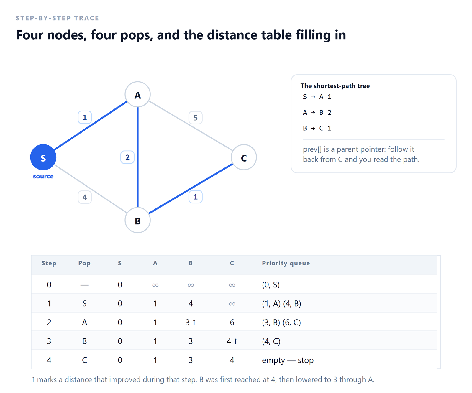
prev[] describes.The trace rewards a close look. At step 1 the queue holds (1, A) and (4, B), so A is popped next even though B was discovered first. That is the greedy choice: the smallest tentative distance goes first. At step 2, A‘s edge to B proposes 3, which beats 4, so B‘s distance is overwritten and a new entry is pushed. The old (4, B) entry is still in the heap and will be skipped later by the stale check.
Relaxation: The Core Operation
Every distance in the algorithm is written by the same three-line test, called relaxation. It asks one question: is the route to v that passes through u cheaper than the best route to v found so far?
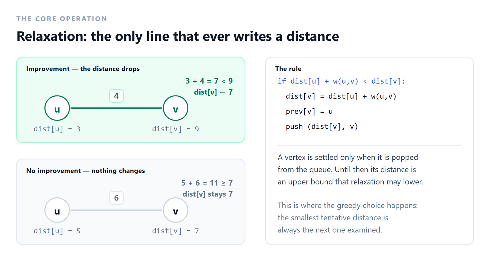
if dist[u] + w(u, v) < dist[v]:
    dist[v] = dist[u] + w(u, v)
    prev[v] = u
    push (dist[v], v) into the queue
The word “relax” is a metaphor: before the test, dist[v] is pulled tight like a stretched spring. If a shorter route exists, the value relaxes down to it. If not, nothing happens.
Three properties of this test deserve attention.
It is strict. The comparison uses <, not <=. When two routes tie, the first one found is kept, which makes the algorithm’s output deterministic for a given input order. Changing it to <= does not break correctness, but it does push extra entries into the queue and can make results depend on traversal order in confusing ways.
It never increases a distance. dist[v] only ever goes down. That monotonicity is why the stale check works: an entry is stale exactly when its stored distance is larger than the current one.
It respects direction. For an undirected graph you add both u → v and v → u to the adjacency list. Forgetting the reverse edge is the single most common bug in hand-written implementations, and it produces a graph that looks right but silently gives wrong answers.
A Complete Worked Example
Here is a six-vertex undirected graph with eight weighted edges. The source is A.
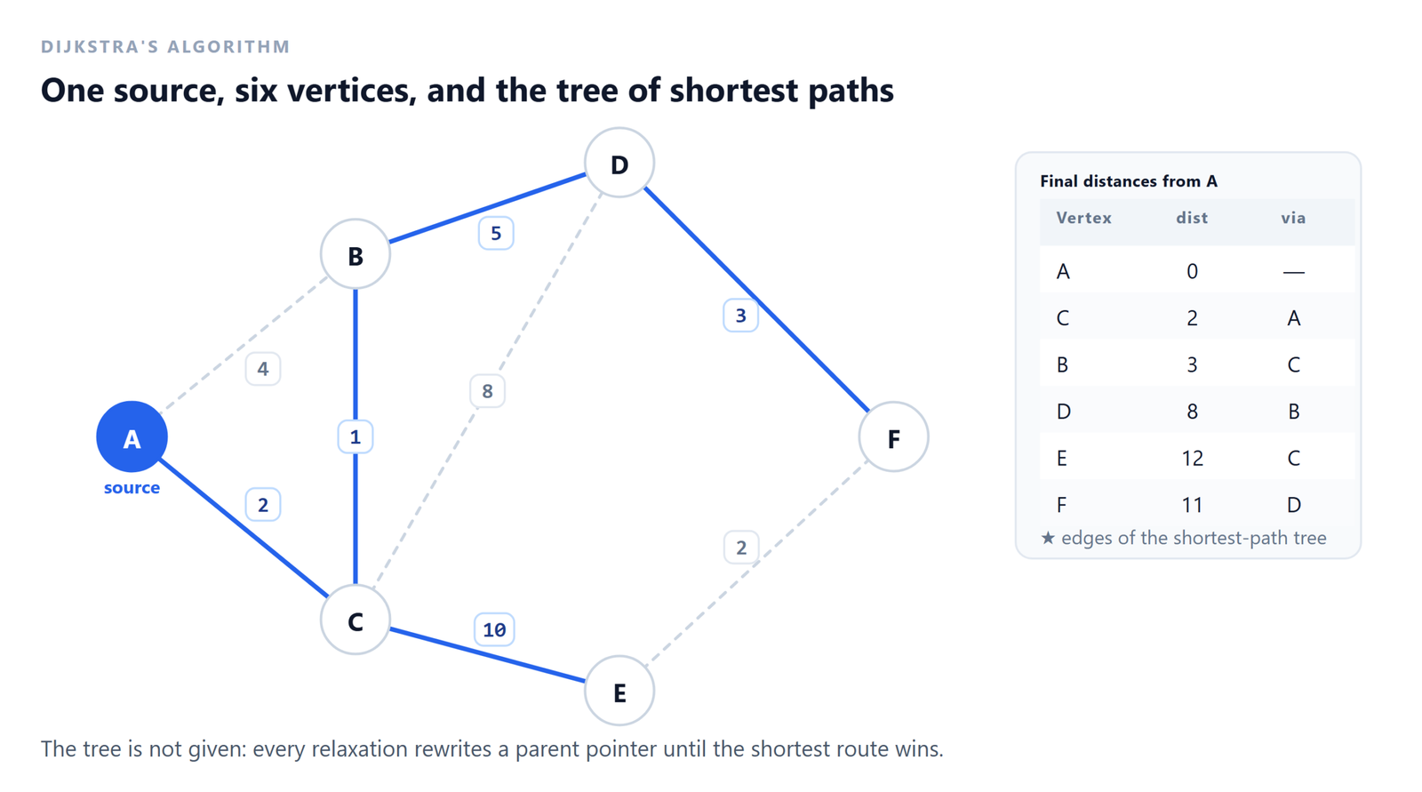
Before running the algorithm, notice that the direct edge A → B costs 4 while the two-edge route A → C → B costs 2 + 1 = 3. A greedy algorithm that simply took the cheapest edge out of the source would pick wrongly here. Dijkstra’s algorithm does not take edges; it settles vertices, which is why it handles this case correctly.
The table records the state after each pop. Distances that changed during that step are marked with an arrow.
| Step | Pop | C | B | D | E | F | Queue afterwards |
|---|---|---|---|---|---|---|---|
| 0 | — | ∞ | ∞ | ∞ | ∞ | ∞ | (0, A) |
| 1 | A (0) | 2 | 4 | ∞ | ∞ | ∞ | (2, C) (4, B) |
| 2 | C (2) | 2 | 3 ↑ | 10 | 12 | ∞ | (3, B) (10, D) (12, E) |
| 3 | B (3) | 2 | 3 | 8 ↑ | 12 | ∞ | (8, D) (12, E) |
| 4 | D (8) | 2 | 3 | 8 | 12 | 11 | (11, F) (12, E) |
| 5 | F (11) | 2 | 3 | 8 | 12 | 11 | (12, E) |
| 6 | E (12) | 2 | 3 | 8 | 12 | 11 | empty — stop |
Reading the trace row by row:
- Step 1. A is settled at 0. Its two edges propose C at 2 and B at 4.
- Step 2. C is the cheapest at 2. Settling it drops B from 4 to 3, and discovers D at 10 and E at 12.
- Step 3. B is now the cheapest at 3. Settling it drops D from 10 to 8, because 3 + 5 beats 2 + 8.
- Step 4. D at 8 is popped and reaches F at 11.
- Step 5. F at 11 beats E at 12, so it is popped first. Its edge to E would give 13, which is worse than 12, so nothing changes.
- Step 6. E is the last vertex. Both of its edges lead to already-settled vertices with no improvement. The queue empties.
The final distances are A = 0, C = 2, B = 3, D = 8, F = 11, E = 12. Following parent pointers from F backwards gives F → D → B → C → A, which reversed is A → C → B → D → F, with total weight 2 + 1 + 5 + 3 = 11.
Notice what did not happen. The algorithm never “changed its mind” about a settled vertex. C was settled at 2 and stayed at 2. B was improved before being settled, while it was still only a candidate. Those two cases — improving an unsettled vertex, and never touching a settled one — are exactly what the correctness proof is about.
Why the Greedy Choice Is Safe
“Pop the cheapest candidate and treat it as final” sounds like a leap of faith. It is not, but the justification requires two short steps.
Lemma: every subpath of a shortest path is shortest
Let P be a shortest path from the source s to some vertex u, and let y be any vertex on P. Then the portion of P from s to y is a shortest path from s to y.
Proof. Suppose the prefix is not shortest. Then some other path Q from s to y is shorter. Replace the prefix of P with Q to obtain a new path from s to u with smaller total weight. That contradicts the assumption that P was shortest. ∎
This is the property that makes incremental construction possible: distances to earlier vertices on a route are independent of the later ones.
Theorem: a popped vertex has its final distance
Assume every edge weight is non-negative. When the algorithm pops a vertex u from the priority queue, dist[u] already equals the true shortest distance d(u).
Proof by induction on the order in which vertices are settled. Let S be the set of vertices already settled before u is popped.
First, dist[u] is always the length of some real path — it was written by a successful relaxation, which follows actual edges from the source. So dist[u] ≥ d(u), and it is enough to rule out dist[u] > d(u).
Suppose dist[u] > d(u), and let P be a genuine shortest path from s to u. Walk along P from s and let y be the first vertex on P that is not in S. Such a vertex exists, because u itself is not in S. Let x be the vertex immediately before y on P; since y is the first unsettled vertex, x is settled.
When x was popped, the algorithm relaxed the edge (x, y). By the induction hypothesis dist[x] = d(x), and by the lemma the prefix of P up to y is a shortest path, so that relaxation set
dist[y] ≤ dist[x] + w(x,y) = d(x) + w(x,y) = d(y).
Distances never increase, so this inequality still holds now. Because all weights are non-negative, the remainder of P from y to u has length at least zero, hence d(y) ≤ d(u). Chaining the three facts:
dist[y] ≤ d(y) ≤ d(u) < dist[u].
So y is an unsettled vertex whose key is strictly smaller than u‘s. But the algorithm popped u as the minimum of the queue. Contradiction. Therefore dist[u] = d(u). ∎
Where the non-negative assumption enters
The proof uses “weights are non-negative” at exactly one place: to conclude d(y) ≤ d(u) from the fact that y lies on a shortest path to u. A negative edge later on that path would make the remaining distance negative, so d(y) could exceed d(u) and the contradiction would collapse. The theorem does not merely lose rigour — it becomes false, as the negative-weight section demonstrates with a concrete graph.
A subtlety the proof exposes. The theorem is about popped vertices. Unsettled vertices can hold distances that are too large — every entry in the queue is a hypothesis, not a fact. That is why “settled” and “discovered” must be kept distinct in code.
Pseudocode
Here is the algorithm in language-independent form. It uses lazy deletion rather than a decrease-key operation, which is what almost every real implementation does.
DIJKSTRA(graph, source)
    for each vertex v in graph
        dist[v] ← INFINITY
        prev[v] ← NONE
    dist[source] ← 0

    pq ← empty min-priority queue
    push (0, source) into pq

    while pq is not empty
        (d, u) ← extract-min(pq)

        if d > dist[u]              # stale entry: skip
            continue

        for each (v, w) in graph[u]  # relax every outgoing edge
            if dist[u] + w < dist[v]
                dist[v] ← dist[u] + w
                prev[v] ← u
                push (dist[v], v) into pq

    return dist, prev
Two implementation choices are hidden in that text.
Lazy deletion instead of decrease-key. A textbook description often says “decrease the key of v in the queue”. Most standard-library heaps cannot do that efficiently, so implementations push a fresh entry and skip the obsolete one when it surfaces. The queue grows to at most E entries, which changes the complexity by a logarithmic factor that is absorbed anyway.
No explicit settled set. With the d > dist[u] guard, a vertex can still be popped twice if its distance is improved after it was settled — an impossible event on valid input, but exactly what happens when a negative edge sneaks in. Adding an explicit settled set makes the intent unambiguous and keeps the behaviour sane on invalid input. The Python version below includes it for that reason.
Python Implementation
The implementation uses heapq from the standard library and an adjacency list stored as a dictionary of lists. It handles disconnected graphs, self-loops and parallel edges without special cases.
import heapq
import math


def dijkstra(graph, source):
    """Return (dist, prev) for shortest paths from source.

    graph: dict mapping a vertex to a list of (neighbour, weight) pairs
    """
    dist = {v: math.inf for v in graph}
    prev = {v: None for v in graph}
    dist[source] = 0

    pq = [(0, source)]        # (distance, vertex)
    settled = set()

    while pq:
        d, u = heapq.heappop(pq)

        if d > dist[u]:
            continue          # stale entry from an older, worse route
        if u in settled:
            continue          # already final, never re-open

        settled.add(u)

        for v, w in graph[u]:
            candidate = d + w
            if candidate < dist[v]:
                dist[v] = candidate
                prev[v] = u
                heapq.heappush(pq, (candidate, v))

    return dist, prev


def path_to(prev, source, target):
    """Rebuild the route as a list of vertices, or [] if unreachable."""
    path = []
    node = target
    while node is not None:
        path.append(node)
        node = prev[node]
    path.reverse()
    return path if path and path[0] == source else []


# --- the graph from the worked example (undirected) ---
edges = [
    ("A", "B", 4), ("A", "C", 2), ("B", "C", 1), ("B", "D", 5),
    ("C", "D", 8), ("C", "E", 10), ("D", "F", 3), ("E", "F", 2),
]

graph = {v: [] for v in "ABCDEF"}
for u, v, w in edges:
    graph[u].append((v, w))
    graph[v].append((u, w))          # reverse edge: the graph is undirected

dist, prev = dijkstra(graph, "A")

for vertex in "ABCDEF":
    route = path_to(prev, "A", vertex)
    print(f"A to {vertex}: {dist[vertex]:>3}  via {' -> '.join(route)}")
Line-by-line explanation
dist = {v: math.inf for v in graph} initialises every distance to infinity. Using the graph’s own keys means the function works for any vertex naming scheme — integers, strings, tuples. math.inf compares correctly against every finite number and needs no special sentinel.
pq = [(0, source)] starts the queue with the source at distance zero. Tuples compare lexicographically, so heapq orders by distance first and breaks ties by vertex name. That tie-breaking matters: if two entries had identical distances and the second element were an unorderable type, the comparison would raise TypeError.
if d > dist[u]: continue is the stale check. Every improvement pushes a new entry without removing the old one, so the heap accumulates history. An entry is obsolete exactly when a strictly better distance has since been recorded.
if u in settled: continue enforces the invariant that a settled vertex is never expanded twice. On a graph with non-negative weights this branch is unreachable; including it turns a silent wrong answer into correct behaviour if the input ever violates the algorithm’s precondition, which is far easier to debug.
for v, w in graph[u] walks the outgoing edges. Because the adjacency list was built with both directions, undirected edges behave correctly without any extra code.
candidate < dist[v] is the relaxation test. The strict inequality keeps the first of two equal routes, which is what makes the output reproducible.
prev[v] = u records the parent. Every successful relaxation rewrites it, so after the loop each vertex points at the neighbour that offered its final distance — and those pointers form a tree.
Testing the implementation
The code above was checked against an independent Bellman-Ford implementation on 300 randomly generated graphs, including graphs with zero-weight edges, self-loops and duplicate edges, and against sorted()-style brute force on small cases. It also handles the boundary cases directly:
- Empty graph with an unknown source raises
KeyErrorimmediately, which is the right behaviour — a source that is not a vertex is a caller error. - Single vertex, no edges returns distance 0 for the source and nothing else.
- Disconnected graph leaves unreachable vertices at infinity, and
path_toreturns an empty list for them because the parent chain never reaches the source. - Self-loop at the source proposes
0 + w, which never beats 0 for non-negativew, so it is ignored. - Parallel edges between the same pair are all relaxed; the cheapest one wins and the others become stale entries.
A correctness trap worth knowing. If you remove the settled guard and only keep the stale check, the code still produces correct answers on non-negative graphs — but on a graph with a negative edge it may accidentally find the right answer by re-expanding vertices, hiding the invalid input instead of exposing it. The guard is what makes the algorithm’s precondition observable.
Reconstructing the Actual Path
Distances alone rarely solve the real problem. The parent pointers give the route, and the reconstruction is a walk backwards:
def path_to(prev, source, target):
    path = []
    node = target
    while node is not None:      # follow parents to the root
        path.append(node)
        node = prev[node]
    path.reverse()               # we collected target -> source
    return path if path and path[0] == source else []
Two details make this robust. The path[0] == source test distinguishes “reached the source” from “fell off the end of a chain that never reached the source”, which is how unreachable vertices appear. And because prev[source] is None, the loop terminates at the root of the tree without needing a separate counter.
A path is at most V vertices long, so reconstruction costs O(V) per query. If you need many routes from the same source, that cost is negligible next to the sort itself — but if you need routes from every source, run the algorithm per source or use an all-pairs method instead.
Time and Space Complexity
Dijkstra’s running time depends on how the priority queue is implemented, and this is where most tutorials give a single number that hides the interesting part.
| Priority queue | Extract-min | Insert / decrease-key | Total time | Notes |
|---|---|---|---|---|
| Unsorted array, linear scan | O(V) | O(1) | O(V² + E) = O(V²) | Best constant factors on dense graphs, trivial to code |
| Binary heap | O(log V) | O(log V) | O((V + E) log V) | The default choice; heapq is this |
| d-ary heap | O(d logd V) | O(logd V) | O((V + E) logd V) | 4-ary heaps beat binary heaps for large graphs |
| Fibonacci heap | O(log V) amortised | O(1) amortised | O(E + V log V) | Theoretically optimal, poor constants, rarely used |
| Pairing heap | O(log V) amortised | O(1) amortised | O(E + V log V) in practice | Similar bounds, much simpler than Fibonacci |
Why the binary-heap bound looks the way it does. Each vertex is extracted at most once, at O(log V). Each edge triggers at most one successful relaxation, and therefore at most one push, at O(log V). That gives O(V log V + E log V), which is normally written O((V + E) log V). Lazy deletion pushes at most E times rather than once per edge relaxation attempt, which is the same order.
Why O(V²) can win anyway. When E is close to V², the heap bound becomes O(V² log V), which is asymptotically worse than a plain array scan. The array version also has no pointer chasing and no heap maintenance, so its constant factor is small. This is the origin of the standard advice to use the array version for dense graphs — advice that, as the next section shows, does not transfer to every language.
Space. The adjacency list costs O(V + E) and the distance, parent and settled arrays cost O(V) each. Total extra space is O(V + E). With an adjacency matrix the graph itself costs O(V²), which usually dominates everything else.
Best, average and worst case are the same. Unlike quicksort, Dijkstra’s algorithm has no input pattern that makes it degenerate. Every vertex is popped once and every edge is relaxed once, regardless of the order in which they appear. The only variation comes from the priority queue, not the data.
Dense vs Sparse: Which Implementation Should You Use?
The textbook rule is simple: sparse graphs want a heap, dense graphs want a matrix scan. The crossover is around E ≈ V² / log V. Below it the heap wins; above it the array scan wins.
That rule is a statement about machine-level constants, and it is worth testing rather than assuming. The table below compares the two implementations on the same machine, in pure Python, taking the best of three runs.
| Graph shape | V | E | Binary heap | O(V²) array scan | Winner |
|---|---|---|---|---|---|
| Complete | 200 | 39,800 | 3.0 ms | 5.5 ms | Heap |
| Complete | 400 | 159,600 | 11.8 ms | 22.4 ms | Heap |
| Sparse, degree ≈ 4 | 1,000 | 7,992 | 2.2 ms | 106.7 ms | Heap |
| Sparse, degree ≈ 4 | 2,000 | 15,982 | 4.7 ms | 448.8 ms | Heap |
| Sparse, degree ≈ 4 | 4,000 | 31,992 | 21.1 ms | 1,910.5 ms | Heap |
The heap version won every case, including complete graphs where the array scan should have the advantage. The reason is that the asymptotic comparison counts memory scans, while Python counts interpreter operations. The array version’s inner loop is bytecode — an index, a bounds check, a None test, a comparison — executed once per matrix cell. The heap version’s hot loop unpacks tuples from a pre-built list, and its push and pop are C functions. The constant factor swamps the logarithmic one.
In C, C++ or Rust the same experiment usually flips on complete graphs, because the array inner loop compiles to a tight contiguous scan while the heap’s operations touch scattered memory. So the practical rule is:
- Pure Python, JavaScript, Ruby: use the heap version unless you have measured otherwise. The array version rarely wins.
- C, C++, Rust, Go: use the array scan when
Eis close toV², and the heap otherwise. Many libraries pick between the two at runtime. - Adjacency matrix already in memory: the array scan is usually right, because the matrix’s own memory cost has already been paid.
- Graph stored as a sparse list: the heap version, because building a matrix just to run the scan would be wasteful.
Measure, then choose. The complexity table tells you how the cost grows. It does not tell you which of two programs finishes first at your input size in your language. Both of these implementations are twenty lines long, so there is no reason to guess.
Why Negative Weights Break It
Dijkstra’s algorithm settles a vertex permanently the moment it is popped. If a later relaxation could still improve that vertex, the commitment would be a mistake. Non-negative weights guarantee that no such improvement can exist. A single negative edge removes the guarantee.
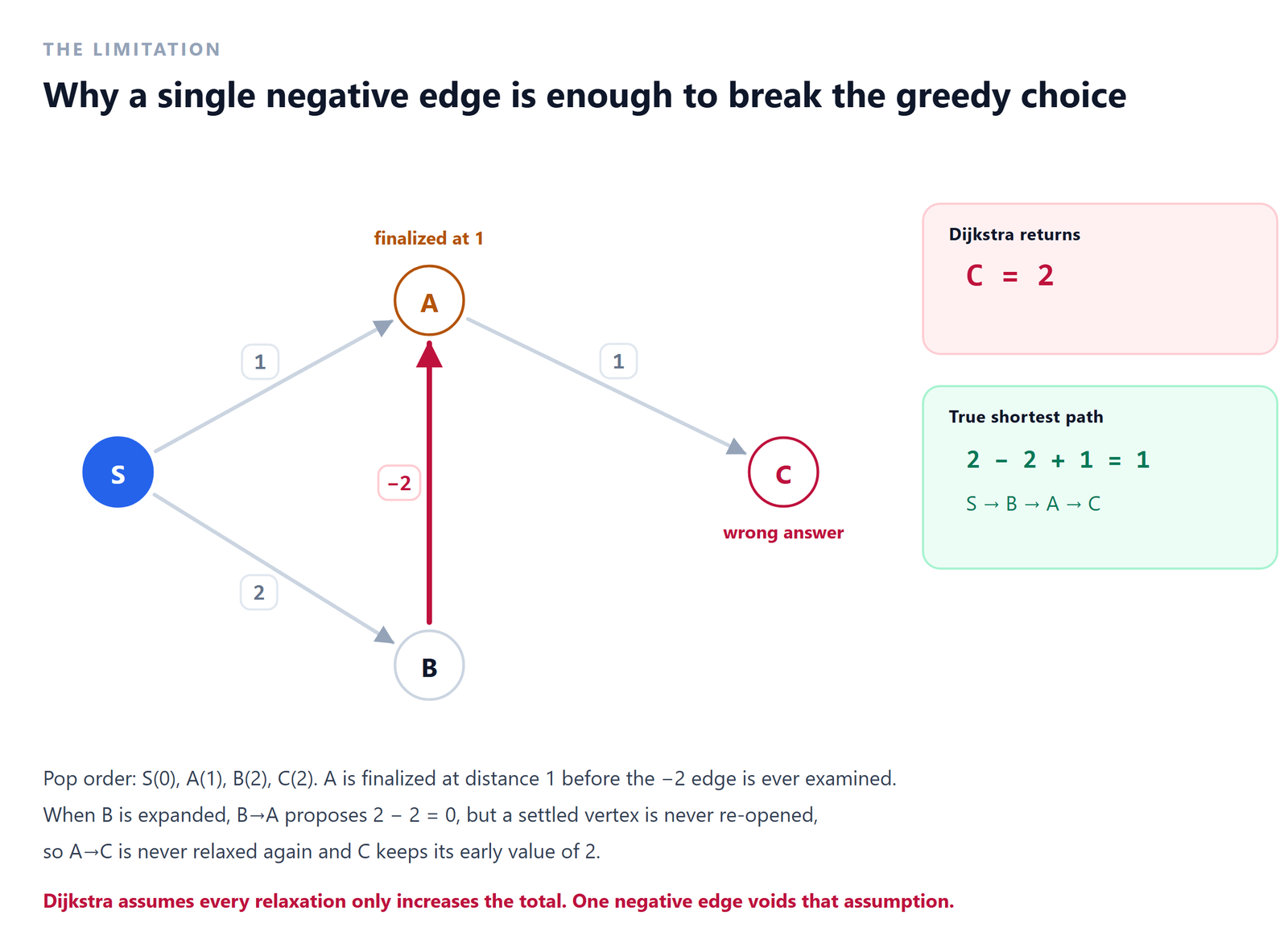
Walk through it slowly, because the failure is subtle. The source is S. The edges are S → A (1), S → B (2), B → A (−2) and A → C (1).
- Pop S (0). Relaxing its edges gives
dist[A] = 1anddist[B] = 2. - Pop A (1). It is the cheapest candidate, so A is settled at 1. Its edge sets
dist[C] = 2. - Pop B (2). Relaxing B → A proposes 2 − 2 = 0, which is better than 1. The distance is overwritten — but A is already settled, so it is never expanded again.
- Pop C (2). No outgoing edges. The queue empties.
The algorithm reports C = 2. The true shortest path is S → B → A → C with length 2 − 2 + 1 = 1. The answer is not merely approximate; it is wrong, and nothing in the output signals that anything went wrong.
The failure happens at the third step. The proof from earlier requires d(y) ≤ d(u) for a vertex y on a shortest path to u. Here A lies on the true shortest path to A itself via B, and the negative edge means the prefix is more expensive than the whole. The inequality that drives the contradiction no longer holds.
The mistake that hides the bug. Some implementations push a new entry whenever a distance improves, without a settled guard. On this graph such code re-expands A and returns the correct answer — by accident, and only because the graph is small. Add another layer of edges behind A and the accident stops happening. If your code gives the right answer here, that is not evidence of correctness; it is evidence that the guard is missing.
What to do instead
Two standard fixes, depending on why the negative weights are there.
Use Bellman-Ford. It relaxes every edge V − 1 times, so it cannot settle anything too early. It runs in O(V·E) rather than O((V + E) log V), and it can detect negative cycles, which Dijkstra’s algorithm cannot. If the graph genuinely has negative weights and no negative cycles, this is the correct tool.
Re-weight the graph. If the negative weights are an artefact of your model rather than a real cost, Johnson’s algorithm re-weights every edge to a non-negative value while preserving shortest-path order, then runs Dijkstra from each vertex. That gives all-pairs shortest paths in O(V·E + V² log V), which beats Floyd-Warshall on sparse graphs.
Never just clamp the negative values to zero. It is a common shortcut and it changes the answer silently. A route that used a negative edge becomes a different route, and the distances reported no longer correspond to any path in the original graph.
Why it cannot detect negative cycles
A negative cycle is a loop whose total weight is negative. Traversing it repeatedly makes the distance to every vertex on the loop arbitrarily small, so “shortest path” is undefined. Bellman-Ford detects this on its final pass: if any edge can still be relaxed after V − 1 rounds, a negative cycle exists. Dijkstra’s algorithm never performs that check, and on a graph containing a negative cycle it simply returns whatever values it happened to settle on before the cycle was encountered.
Dijkstra vs Other Algorithms
Four comparisons matter in practice. Each answers a different question, and choosing the wrong one is a design error rather than an optimisation mistake.
Dijkstra vs Bellman-Ford vs Floyd-Warshall
| Dijkstra | Bellman-Ford | Floyd-Warshall | |
|---|---|---|---|
| Answers | One source, all targets | One source, all targets | All pairs |
| Negative edge weights | No | Yes | Yes |
| Detects negative cycles | No | Yes | Yes |
| Time | O((V + E) log V) with a heap | O(V · E) | O(V³) |
| Space | O(V + E) | O(V + E) | O(V²) |
| Best for | Large graphs, non-negative weights | Negative edges, one source | Small graphs, all pairs, negative edges |
On a sparse graph with 10,000 vertices and 40,000 edges, Dijkstra takes roughly (40,000 + 10,000) × 13 ≈ 650,000 heap steps, Bellman-Ford takes 400 million relaxations, and Floyd-Warshall would need 1012 operations. The gap is not a constant factor; it is the difference between a runnable program and an unusable one.
Dijkstra vs BFS
BFS is Dijkstra’s algorithm with every weight equal to 1. It uses a plain FIFO queue instead of a heap, runs in O(V + E), and is strictly better when the graph is genuinely unweighted. Using Dijkstra on an unweighted graph is correct but wasteful — it pays a logarithmic factor for ordering that BFS gets for free.
A useful middle case: if every edge weight is a small integer, you can expand each edge of weight w into w unit edges and use BFS, or replace the heap with a bucket queue (Dial’s algorithm) for O(V + E + max weight).
Dijkstra vs A*
A* search is Dijkstra’s algorithm plus a heuristic that estimates the remaining distance to a specific target. Instead of ordering by dist[u], it orders by dist[u] + h(u). With an admissible heuristic — one that never overestimates — A* returns the same optimal path while expanding far fewer vertices. With h = 0 it degenerates exactly to Dijkstra.
Use Dijkstra when you need distances to many targets, and A* when you need one target and can define a good heuristic. That is why routing engines use A* or its variants for point-to-point queries but Dijkstra for building a full distance table.
Dijkstra vs Prim’s algorithm
Both grow a tree by repeatedly selecting a vertex with a priority queue, so the code looks almost identical. The key differs:
- Dijkstra orders candidates by
dist[source][u]— the cost of the whole route from the source. - Prim orders candidates by
w(u, parent)— the cost of the single edge joininguto the tree.
Changing one line converts one algorithm into the other. The outputs are different objects: a shortest-path tree versus a minimum spanning tree. A minimum spanning tree can contain a route between two vertices that is much longer than the shortest path between them.
Edge Cases and Common Bugs
Most broken implementations fail in one of the ways below. Each has a characteristic symptom.
| Bug | Symptom | Fix |
|---|---|---|
| Missing the reverse edge for an undirected graph | Some vertices report infinity, or paths exist in only one direction | Add both (v, w) to graph[u] and (u, w) to graph[v] |
| No stale-entry check | Distances are sometimes too small, or extra edges get relaxed from outdated values | Skip when d > dist[u] |
| No settled guard | Correct on valid input, silently re-expands on invalid input | Keep a settled set |
Using <= in the relaxation test |
Correct but pushes duplicate work; path choice becomes order-dependent | Use strict < |
| Comparing tuples whose second element is unorderable | TypeError when two distances tie |
Add a counter as the middle element: (d, i, v) |
Initialising dist with a large integer like 109 |
Overflow or wrong answers when real paths exceed the sentinel | Use math.inf or a value provably larger than any path |
| Treating 0-weight edges as absent | Valid zero-cost routes are missed | Test explicitly for None, not for falsiness |
| Running on a graph with negative weights | Plausible but wrong distances, no error | Use Bellman-Ford, or re-weight first |
Assuming prev[target] is always reachable |
Infinite loop or empty path on disconnected graphs | Check that the chain ends at the source |
| Mutating the graph while iterating | Edges are silently skipped | Collect edge updates first, then apply them |
A one-line test that catches most of them: take a graph, run the algorithm from every vertex, and check that dist[u][v] == dist[v][u] for undirected input. Asymmetry exposes a missing reverse edge instantly. Then add a single negative edge and confirm that your code either refuses the input or produces the documented wrong answer — if it quietly produces a correct answer, you are missing the settled guard.
Self-loops, parallel edges, zero weights and empty graphs
Self-loops (u → u) are harmless: they propose dist[u] + w, which never beats dist[u] when w ≥ 0. A negative self-loop is a negative cycle, and the algorithm misbehaves exactly as the previous section describes.
Parallel edges between the same pair are fine — the cheapest one wins and the others become stale entries that the queue discards.
Zero-weight edges are valid input. They create ties, which the strict inequality resolves by keeping the first route found. A graph made entirely of zero-weight edges still produces a correct spanning tree of reachable vertices.
An empty graph or a source that is not a vertex is a caller error, not a graph property. Fail fast with an exception rather than returning a partially initialised result.
Applications of Dijkstra’s Algorithm
The algorithm’s reach is wider than “maps”, though that is where it started.
- Route planning. Road networks, public transport timetables and delivery dispatch all run Dijkstra or a variant. Production systems usually add A*, contraction hierarchies or landmark-based preprocessing, but Dijkstra is the reference implementation they are validated against.
- Network routing. Link-state protocols such as OSPF compute shortest paths across a network topology. Each router runs Dijkstra on the topology it has learned, which is why convergence after a topology change is fast and predictable.
- Social and citation graphs. Degrees of separation, influence propagation and recommendation explanations are weighted shortest-path problems.
- Game AI. Navigation meshes and grid maps are searched with Dijkstra or A*, often with terrain costs encoded as edge weights.
- Currency and arbitrage detection. Convert exchange rates to negative logarithms and shortest paths become the cheapest conversion chain. A negative cycle is an arbitrage opportunity, which is why that case needs Bellman-Ford rather than Dijkstra.
- Puzzle solving. Any state-space search with non-uniform step costs — word ladders with letter costs, sliding puzzles with move penalties — is a shortest-path problem.
- Image processing. Seam carving, graph-cut segmentation and geodesic distance transforms all rely on shortest paths over pixel grids.
- Compilers and build systems. Critical-path analysis and dependency scheduling use the same relaxation mechanism on a DAG.
It is the wrong tool when weights can be negative, when the graph is small enough that a simple search is clearer, or when you need a minimum spanning tree rather than shortest paths.
Variants and Optimisations
Production implementations of Dijkstra are recognisably the same algorithm with several of the following changes.
Early exit for a single target. If you only need the distance to one vertex, stop as soon as that vertex is popped. On a road network this can cut the explored area dramatically, because Dijkstra otherwise expands outward in every direction equally.
Bidirectional search. Run a forward search from the source and a backward search from the target, alternating between them, and stop when their frontiers meet. Correctness requires care — the meeting vertex is not necessarily on the optimal path — but the explored region shrinks from roughly a disc to a narrow ellipse. On road networks this is a large practical win.
A* and its variants. Adding an admissible heuristic turns the search toward the target without sacrificing optimality. Landmark-based heuristics (ALT) precompute distances to a few chosen vertices and use the triangle inequality to derive strong bounds.
Contraction hierarchies. Preprocess the graph by repeatedly contracting the least important vertex, producing a hierarchy that allows queries in microseconds on continental road networks. This is what most commercial routing engines use, and it is built on top of bidirectional Dijkstra.
Dial’s algorithm (bucket queue). When edge weights are small integers, replace the heap with an array of buckets indexed by distance. Extract-min becomes a pointer advance and the running time drops to O(V + E + C), where C is the largest distance. This is a genuine improvement, not a constant-factor tweak.
Graph compression. Removing degree-2 vertices and merging short chains reduces the graph before the search ever starts. The compressed graph is smaller, and the removed segments are re-expanded afterwards.
Parallel and GPU implementations. Delta-stepping processes buckets of vertices concurrently, and GPU variants exploit the fact that relaxation is data-parallel. These matter at the scale of billions of edges.
Every one of these is an optimisation on top of the same core loop. If you understand the pop-settle-relax cycle, you understand all of them.
Frequently Asked Questions
Is Dijkstra’s algorithm greedy?
Yes. At every step it makes the locally optimal choice — settle the unsettled vertex with the smallest tentative distance — and never reconsiders. What makes it unusual is that this greedy choice is provably optimal, but only when all edge weights are non-negative.
Can Dijkstra’s algorithm handle negative edge weights?
No, not reliably. A negative edge can make a route to an already-settled vertex cheaper after it has been finalised, and the algorithm never re-opens settled vertices. The result is a wrong distance with no error reported. Use Bellman-Ford for graphs with negative weights, or re-weight the edges first with Johnson’s algorithm.
Why exactly does Dijkstra fail with negative edges?
Because the correctness proof needs the remaining part of a path to have non-negative length, so that a vertex early on a shortest path cannot be more expensive than the destination. A negative edge breaks that inequality. Concretely, with edges S to A of 1, S to B of 2 and B to A of minus 2, the algorithm settles A at 1 before discovering that the route through B costs 0.
Dijkstra vs Bellman-Ford: which should I use?
Use Dijkstra when all weights are non-negative and the graph is large, because it runs in O((V + E) log V) against Bellman-Ford’s O(V · E). Use Bellman-Ford when negative weights are possible, when you need to detect a negative cycle, or when the graph is distributed across routers that exchange edge information asynchronously.
What is the time complexity of Dijkstra’s algorithm?
It depends on the priority queue. With a binary heap it is O((V + E) log V). With a plain array and linear scan of the minimum it is O(V² + E), which simplifies to O(V²) on dense graphs. With a Fibonacci heap it is O(E + V log V). Space is O(V + E) with an adjacency list, or O(V²) with an adjacency matrix.
Does Dijkstra’s algorithm work on directed graphs?
Yes, and directed graphs are the natural case — the algorithm only ever follows edges in their forward direction. For undirected graphs you simply store each edge twice, once in each adjacency list. Nothing else in the algorithm changes.
Is BFS better than Dijkstra for unweighted graphs?
Yes. When every edge has the same weight, BFS finds shortest paths in O(V + E) using a plain queue, while Dijkstra pays an extra logarithmic factor for ordering it does not need. Dijkstra is the generalisation of BFS to weighted edges.
Why does Dijkstra need a priority queue?
Because the algorithm’s correctness depends on always settling the cheapest candidate next. A priority queue returns that minimum efficiently. With a plain queue you would settle vertices in arrival order, which is exactly the greedy choice that weighted edges invalidate.
Does Dijkstra always find the shortest path?
It finds the shortest path from the source to every reachable vertex, provided all edge weights are non-negative and the graph has no negative cycles. Unreachable vertices correctly remain at infinity. If negative weights are present, the answer may be wrong even though the algorithm completes without complaint.
What is the difference between Dijkstra and A*?
A* orders candidates by distance travelled plus an estimate of the remaining distance to a specific target, while Dijkstra orders only by distance travelled. With an admissible heuristic, A* returns the same optimal path after exploring fewer vertices. Dijkstra remains better when you need distances to many targets at once.
Dijkstra or Prim’s algorithm?
Dijkstra builds a shortest-path tree: it minimises the distance from the source to each vertex. Prim’s algorithm builds a minimum spanning tree: it minimises the total weight of the edges used. The code differs by a single line — the priority key — but the outputs answer different questions and are usually different trees.
Can Dijkstra detect negative cycles?
No. It never re-examines a settled vertex, so it cannot notice that a loop keeps lowering distances. Only Bellman-Ford and Floyd-Warshall detect negative cycles, by checking on a final pass whether any edge can still be relaxed.
What happens when two vertices have the same distance?
Either may be settled first, and both orders produce correct distances. The tie only changes which of several equally short paths is reported. In Python, tuples compare by their second element, so the vertex name breaks the tie deterministically — but if the vertex type is not orderable you must add an explicit counter to avoid a TypeError.
Practice Problems
These exercises target the parts of the algorithm that tutorials usually skip. They need no particular platform.
- Trace by hand. Run the algorithm on the six-vertex graph in this article starting from D instead of A. Write down the pop order and the queue after every step, then check your answer with the Python code.
- Prove the subpath lemma. The proof in this article is two sentences. Rewrite it formally for a directed graph, stating exactly where the assumption that P is shortest is used.
- Break it on purpose. Add a single negative edge to the worked example and find an input where the algorithm reports a wrong distance. Then confirm Bellman-Ford gets it right.
- Count the pushes. Instrument the implementation to count heap pushes for random graphs of increasing density. Verify that the count never exceeds E and explain why.
- Implement the array version. Write the O(V²) adjacency-matrix variant and confirm it matches the heap version on random graphs. Then benchmark both at V = 200, 400 and 800 on complete graphs.
- Add an early exit. Modify the implementation to stop as soon as a target vertex is popped. Prove that the returned distance is still optimal.
- Dial’s algorithm. Replace the heap with an array of buckets for integer weights in the range 0 to 20. Measure the speedup at V = 10,000.
- Path counting. Extend the algorithm to count how many distinct shortest paths exist between the source and each vertex. Watch out for ties.
Conclusion
Dijkstra’s algorithm is one of the small number of results in computer science that are simultaneously obvious in hindsight and genuinely deep. Its loop is six lines: initialise, push, pop, settle, relax, repeat. Its guarantee rests on a single assumption, and understanding that assumption is what separates using the algorithm from trusting it blindly.
The mechanism is worth restating in one sentence: because every prefix of a shortest path is itself a shortest path, and because non-negative weights prevent a later edge from undercutting an earlier one, the cheapest unsettled candidate can be finalised on the spot. Every property of the algorithm follows from that sentence — its correctness, its complexity, and its one fatal limitation.
The limitation is not a technicality. One negative edge turns a correct program into a confidently wrong one, with no exception and no warning. That is why the negative-weight case deserves more than a footnote, and why so many real systems either forbid negative weights at the type level or fall back to Bellman-Ford when they cannot.
The practical lessons are less glamorous but more useful. Choose the priority queue by measuring rather than by reciting the textbook rule — in Python the heap won even on complete graphs. Keep the stale-entry check and the settled guard, because they document the invariant and expose invalid input. Store undirected edges in both directions. Use math.inf rather than a large integer. And remember that the distances are half the answer; the parent pointers are what let you act on them.
If you want to see how the same ideas appear elsewhere, the A* search algorithm adds a heuristic to this exact loop, Prim’s algorithm changes one priority key to build a spanning tree instead, and radix sort shows a different way to escape a complexity lower bound by exploiting structure in the keys. More algorithm guides are collected in the Algorithm category.