Gradient Boosting in Machine Learning: How It Works

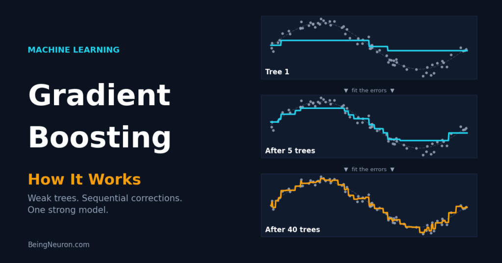
Gradient boosting builds a strong predictor by adding many small, simple decision trees one after another, where each new tree is trained to correct the errors left by all the trees before it. It is one of the most accurate methods for tabular data, and it powers libraries such as XGBoost, LightGBM, and CatBoost that dominate machine learning competitions and many production systems.

This guide explains how gradient boosting works from first principles: residuals, the gradient view, and the update rule. You will follow a five-sample example by hand, then build classification and regression models in scikit-learn, watch overfitting appear tree by tree, tune the key hyperparameters, and learn which mistakes to avoid.

What Is Gradient Boosting?

Gradient boosting belongs to the family of ensemble methods: techniques that combine many models into one. It uses weak learners, usually shallow decision trees with only a few splits. One shallow tree is a poor predictor. A few hundred of them, each fixing the previous mistakes, form a very accurate one.

The name has two parts. Boosting means models are trained in sequence, each focused on what the earlier ones got wrong. Gradient means the “what they got wrong” is measured by the gradient (slope) of a loss function, which lets the same recipe work for regression, classification, and ranking.

Boosting vs Bagging

Random Forest uses bagging: it trains many deep trees independently on random samples and averages them, which reduces variance. Boosting trains shallow trees sequentially and adds them, which reduces bias.

Bagging: parallel independent trees averaged. Boosting: sequential trees summed.Bagging (Random Forest): parallelBoosting: sequentialDeep tree 1Deep tree 2Deep tree 3Average votesIndependent trees reduce varianceShallowtree 1Shallowtree 2Shallowtree 3errorserrorsPrediction = F₀ + ν(tree 1 + tree 2 + tree 3 + …)Each tree fixes what the earlier ones missed

How Gradient Boosting Works

1. Start with a constant prediction F₀. For regression with squared error it is the mean of the targets.
2. Compute the residuals: the difference between the true target and the current prediction for every training sample.
3. Fit a small tree h₁ that predicts those residuals from the features.
4. Update the model by adding a fraction of the tree: F₁ = F₀ + ν · h₁.
5. Repeat steps 2 to 4 for M rounds. The final model is the sum of all trees.

Initial prediction, then a loop of residuals, tree fitting and model update, producing the final additive model.The boosting loopStartF₀ = mean(y)1. Residualsr = y − F2. Fit small treeh to predict r3. UpdateF = F + ν·hrepeat M timesFinal model: F = F₀ + ν(h₁ + h₂ + … + hM)

The Mathematics Behind Gradient Boosting

The Additive Model

F_m(x) = F_m−1(x) + ν · h_m(x)

• F_m(x) is the model’s prediction for input x after m trees.
• h_m(x) is the m-th tree.
• ν (nu) is the learning rate or shrinkage, between 0 and 1. Small values make each tree contribute less.

Why It Is Called Gradient Boosting

We want to minimize a loss function L(y, F) summed over all samples, where y is the true value and F the prediction. In ordinary gradient descent we adjust parameters against the gradient. In gradient boosting we adjust the predictions themselves. The direction in which each prediction should move is the negative gradient of the loss:

r_i = − ∂L(y_i, F(x_i)) / ∂F(x_i)

These values r_i are called pseudo-residuals. Each new tree is fitted to predict them. The tree learns the pattern in how predictions should change, rather than the changes for single samples, so it generalizes to new inputs.

Case 1: Regression with Squared Error

For L = ½(y − F)², the derivative with respect to F is F − y, so the pseudo-residual is r = y − F: the ordinary residual. That is why the simplified description “fit a tree to the errors” is exact for squared error.

Case 2: Binary Classification with Log Loss

The model predicts a log-odds score F, and the probability is p = 1 / (1 + e^−F). The log loss is L = −[y log p + (1 − y) log(1 − p)], and its negative gradient with respect to F is again simple:

r = y − p

Here y is 0 or 1 and p is the current predicted probability. A positive sample predicted at p = 0.2 has residual 0.8, so the next tree pushes it up strongly. The initial prediction F₀ is the log-odds of the positive class rate. Trees are fitted to these residuals and their leaf values are adjusted to approximate the log-loss optimum. The trees always output numbers on the log-odds scale, which are then turned into probabilities by the sigmoid function.

A Worked Example You Can Check by Hand

Five training points with one feature: x = 1, 2, 3, 4, 5 and targets y = 3, 5, 4, 8, 10. Use squared error, stumps (trees with one split), and learning rate ν = 0.5.

Round 0. F₀ = mean(y) = 6.0 for every sample. The residuals are −3, −1, −2, +2, +4, and the mean squared error (MSE) is (9 + 1 + 4 + 4 + 16) / 5 = 6.8.

Round 1. The best stump splits between x = 3 and x = 4. The left group has residuals −3, −1, −2 with mean −2. The right group has +2, +4 with mean +3. The tree predicts −2, −2, −2, +3, +3. Update: F₁ = 6 + 0.5 × (−2, −2, −2, 3, 3) = (5, 5, 5, 7.5, 7.5). The new residuals are (−2, 0, −1, 0.5, 2.5) and the MSE drops to 2.3.

Round 2. The best stump splits between x = 4 and x = 5. It predicts −0.625 for the first four samples and +2.5 for the last. Update: F₂ = (4.6875, 4.6875, 4.6875, 7.1875, 8.75). The MSE drops to 1.128.

Round 3. The best stump isolates x = 1. It predicts −1.6875 for the first sample and +0.4219 for the other four. F₃ = (3.84, 4.90, 4.90, 7.40, 8.96) and the MSE is 0.594.

Predictions F0, F1 and F3 against the targets 3, 5, 4, 8, 10, and the mean squared error after each round.The prediction approaches the dataMean squared error per round0510x=1x=2x=3x=4x=5dataF₀F₁F₃6.802.301.130.59Round 0Round 1Round 2Round 3Learning rate 0.5, stumps, squared error

This is the full algorithm. Real implementations differ only in using deeper trees, smaller learning rates, and hundreds of rounds. To check this by code, fit DecisionTreeRegressor(max_depth=1) to the residuals in a loop; the printed MSE values match the numbers above (6.8, 2.3, 1.1281, 0.5942).

Key Hyperparameters

Parameter (scikit-learn)	Default	What it controls
n_estimators	100	Number of trees (rounds M). More trees fit the training data more closely.
learning_rate	0.1	Shrinkage ν. Lower values need more trees but usually generalize better.
max_depth	3	Depth of each tree. Controls how many feature interactions one tree can capture.
subsample	1.0	Fraction of rows used per tree. Values like 0.8 add randomness and reduce overfitting (stochastic gradient boosting).
min_samples_leaf	1	Minimum samples in a leaf. Larger values smooth the model.
max_features	None	Features considered per split, as in Random Forest.
n_iter_no_change	None	Early stopping: stop when the validation score has not improved for this many rounds.
loss	log_loss / squared_error	Loss function to minimize. Regression also supports absolute_error and huber, which resist outliers.

learning_rate and n_estimators trade off against each other: halving the learning rate roughly requires doubling the trees for a similar fit. A common strategy is to fix a small learning rate (0.05 to 0.1), set a large n_estimators, and let early stopping find the right number of trees.

Gradient Boosting Classifier in Python

The task: classify tumors as malignant or benign on the Breast Cancer dataset (569 samples, 30 features). Unlike KNN and SVM, tree-based boosting needs no feature scaling.

Step 1: Train a baseline model

from sklearn.datasets import load_breast_cancer
from sklearn.model_selection import train_test_split
from sklearn.ensemble import GradientBoostingClassifier

data = load_breast_cancer()
X_train, X_test, y_train, y_test = train_test_split(
    data.data, data.target, test_size=0.25, random_state=42, stratify=data.target
)

gb = GradientBoostingClassifier(random_state=42)   # 100 trees, depth 3, lr 0.1
gb.fit(X_train, y_train)
print("Test accuracy:", round(gb.score(X_test, y_test), 3))

Output:

Test accuracy: 0.958

Step 2: See how hyperparameters change the result

configs = [(0.1, 100, 3), (0.01, 100, 3), (0.1, 300, 3),
           (0.1, 100, 1), (0.1, 100, 6), (0.05, 500, 3)]

print("lr     trees  depth  train   test")
for lr, n, depth in configs:
    m = GradientBoostingClassifier(learning_rate=lr, n_estimators=n,
                                   max_depth=depth, random_state=42)
    m.fit(X_train, y_train)
    print(f"{lr:<6} {n:<6} {depth:<6} {m.score(X_train, y_train):.3f}  "
          f"{m.score(X_test, y_test):.3f}")

Output:

lr     trees  depth  train   test
0.1    100    3      1.000  0.958
0.01   100    3      0.988  0.937
0.1    300    3      1.000  0.958
0.1    100    1      0.988  0.958
0.1    100    6      1.000  0.944
0.05   500    3      1.000  0.958

Six configurations of learning rate, trees and depth on the Breast Cancer data.Training vs test accuracy by configuration1.000.970.940.911.0000.9580.9880.9371.0000.9580.9880.9581.0000.9441.0000.958lr 0.1100 trees, d3lr 0.01100 trees, d3lr 0.1300 trees, d3lr 0.1100 trees, d1lr 0.1100 trees, d6lr 0.05500 trees, d3TrainTestAxis starts at 0.91

Observations: a learning rate of 0.01 with 100 trees has not finished learning (train 0.988). Depth-6 trees reach perfect training accuracy but lose one test point against depth 3. Stumps (depth 1) already reach 0.958, so on this dataset the interactions between features are not complex. Differences of 1 to 3 test samples should not drive decisions; compare candidates with cross-validation.

Step 3: Early stopping

gb = GradientBoostingClassifier(
    n_estimators=500,           # upper limit
    learning_rate=0.05,
    subsample=0.8,              # each tree sees 80% of the rows
    n_iter_no_change=10,        # stop if validation loss stalls for 10 rounds
    validation_fraction=0.1,    # 10% of training data held out internally
    random_state=42,
)
gb.fit(X_train, y_train)
print("Trees actually built:", gb.n_estimators_)
print("Test accuracy:", round(gb.score(X_test, y_test), 3))

Output:

Trees actually built: 86
Test accuracy: 0.958

Training stopped after 86 of the allowed 500 trees. The attribute n_estimators_ holds the number actually used. Early stopping saves time and protects against overfitting without manual tuning.

Step 4: Feature importance

import numpy as np
order = np.argsort(gb.feature_importances_)[::-1][:5]
for i in order:
    print(f"{data.feature_names[i]:25s} {gb.feature_importances_[i]:.3f}")

Output:

worst concave points      0.415
worst radius              0.126
worst area                0.119
worst perimeter           0.099
mean concave points       0.093

Gradient boosting with early stopping on the Breast Cancer dataset.Which features drive the predictions?worst concave pointsworst radiusworst areaworst perimetermean concave points0.4150.1260.1190.0990.093

These are impurity-based importances. They can favor features with many distinct values and split credit among correlated features. For a more reliable view use sklearn.inspection.permutation_importance on held-out data.

Gradient Boosting Regressor and the Overfitting Curve

Regression uses GradientBoostingRegressor. The Diabetes dataset (442 patients, 10 features) predicts disease progression after one year. Scikit-learn’s staged_predict returns the prediction after each tree, which lets us watch the error shrink and then grow.

from sklearn.datasets import load_diabetes
from sklearn.ensemble import GradientBoostingRegressor
from sklearn.metrics import mean_squared_error

Xd, yd = load_diabetes(return_X_y=True)
Xd_tr, Xd_te, yd_tr, yd_te = train_test_split(Xd, yd, test_size=0.25, random_state=42)

reg = GradientBoostingRegressor(n_estimators=200, learning_rate=0.1,
                                max_depth=3, random_state=42)
reg.fit(Xd_tr, yd_tr)

train_mse = [mean_squared_error(yd_tr, p) for p in reg.staged_predict(Xd_tr)]
test_mse  = [mean_squared_error(yd_te, p) for p in reg.staged_predict(Xd_te)]

print("trees  train_MSE  test_MSE")
for n in [1, 5, 10, 25, 50, 100, 150, 200]:
    print(f"{n:5d}  {train_mse[n-1]:9.0f}  {test_mse[n-1]:8.0f}")
best = int(np.argmin(test_mse)) + 1
print("Best number of trees:", best, "with test MSE", round(min(test_mse)))

Output:

trees  train_MSE  test_MSE
    1       5459      5146
    5       3940      3993
   10       2993      3297
   25       1944      2989
   50       1395      3087
  100        905      3184
  150        572      3270
  200        379      3343
Best number of trees: 27 with test MSE 2971

Training MSE keeps falling while test MSE bottoms out near 27 trees.Boosting keeps fitting the training data, test error turns up6000400020000150100150200Number of treesBest: 27 trees, test MSE 2971Training MSETest MSE

rmse = np.sqrt(test_mse[-1])
print("RMSE with 200 trees:", round(rmse, 2))
print("RMSE of predicting the mean:", round(yd_te.std(), 2))

Output:

RMSE with 200 trees: 57.82
RMSE of predicting the mean: 74.36

Even the overfitted 200-tree model beats the “always predict the average” baseline (57.8 against 74.4), and it beats a single depth-3 decision tree, whose test MSE is 3512 against 3343. The 27-tree model does better still (MSE 2971, RMSE about 54.5). Choosing the number of trees by validation error, with n_iter_no_change or staged_predict, is the single most important tuning step.

Regularization: How to Stop Boosting from Overfitting

• Shrinkage: a small learning_rate (0.01 to 0.1) with more trees.
• Tree constraints: shallow trees (max_depth 2 to 5), larger min_samples_leaf.
• Subsampling: subsample below 1.0 and max_features below 1.0 add randomness.
• Early stopping: halt when validation loss stops improving.
• Robust losses: huber or absolute_error limit the pull of outliers in regression.

XGBoost, LightGBM, CatBoost, and HistGradientBoosting

Scikit-learn’s classic GradientBoosting* classes are clear and easy to use but slow on large data. Modern libraries use the same boosting idea with engineering improvements:

Library	Notable features
HistGradientBoostingClassifier (scikit-learn)	Bins features into histograms for speed, handles missing values natively, early stopping is built in.
XGBoost	Uses second-order gradient information, explicit L1/L2 regularization on leaf values, parallel tree construction, handles missing values.
LightGBM	Histogram-based, grows trees leaf-wise, very fast on large datasets.
CatBoost	Handles categorical features directly and uses ordered boosting to reduce target leakage.

from sklearn.ensemble import HistGradientBoostingClassifier

hgb = HistGradientBoostingClassifier(learning_rate=0.1, max_iter=300,
                                     early_stopping=True, random_state=42)
hgb.fit(X_train, y_train)

For datasets above roughly 10,000 rows, prefer HistGradientBoosting* or LightGBM over the classic estimator.

Gradient Boosting vs Random Forest

Aspect	Gradient Boosting	Random Forest
Tree building	Sequential	Parallel, independent
Tree depth	Shallow (weak learners)	Deep
Main effect	Reduces bias	Reduces variance
Overfitting risk	Higher; needs tuning and early stopping	Lower; robust with defaults
Tuning effort	More	Less
Typical accuracy on tabular data	Often higher when tuned	Strong baseline

Advantages and Disadvantages

Advantages

• High accuracy on structured, tabular data.
• No feature scaling needed; handles mixed feature types and non-linear relationships.
• Works with many loss functions for regression, classification, and ranking.
• Provides feature importance, and modern versions handle missing values.

Disadvantages and Limitations

• Sequential training is slower than Random Forest and cannot be parallelized across trees.
• Sensitive to hyperparameters, and prone to overfitting without early stopping.
• Sensitive to noisy labels and outliers, because later trees try to fit the remaining errors, noise included.
• Less interpretable than a single tree or a linear model.
• Cannot extrapolate beyond the range of training targets, since predictions are sums of leaf values.
• Typically trails deep learning on images, audio, and text.

Common Mistakes and How to Fix Them

Using too many trees with no early stopping

Figure 6 shows test error rising after 27 trees. Use n_iter_no_change or staged_predict.

Using a large learning rate with a small tree count, or the reverse

Lower learning rates need more trees. Fix one, tune the other.

Making trees too deep

Boosting works with weak learners. Start at max_depth 3, and try 2 to 5.

Judging with training accuracy

Training accuracy is 1.000 in most rows of Step 2. Use validation data or cross-validation.

Tuning on the test set

Choose hyperparameters with cross-validation on the training data. Use the test set once.

Ignoring class imbalance

Use stratified splits, sample_weight in fit, and metrics such as F1 or ROC AUC.

Trusting impurity-based feature importance blindly

Verify with permutation importance on held-out data.

ValueError: Input contains NaN

The classic GradientBoosting* estimators do not accept missing values in older versions. Impute them, or use HistGradientBoosting*, XGBoost, or LightGBM, which handle NaN natively.

ValueError: could not convert string to float

Encode categorical columns (one-hot or ordinal) first, or use CatBoost, which accepts categories directly.

Expecting predictions outside the training range

Tree models cannot extrapolate. For trends that continue beyond the data, combine boosting with a linear model or model the residuals of a trend.

Real-World Applications

• Credit risk and fraud detection: gradient boosted trees are a standard model for scoring tabular transaction and customer data.
• Search ranking: boosted trees with ranking losses (LambdaMART) have long been used to order results.
• Customer churn and marketing response: mixed numeric and categorical features suit tree ensembles.
• Demand forecasting and pricing: regression boosting on engineered lag and calendar features.
• Healthcare risk scores: predicting outcomes from lab values and history, as in the tumor example.
• Data science competitions: XGBoost, LightGBM, and CatBoost are frequent winners on tabular tasks.

Related reading on BeingNeuron: Cross-Validation: K-Fold Explained, Support Vector Machines: How They Work, K-Nearest Neighbors Algorithm Explained, and Feature Scaling: Normalization vs Standardization.

Frequently Asked Questions

How does gradient boosting work?

It starts with a simple prediction, then repeatedly fits a small decision tree to the current errors (the negative gradient of the loss) and adds a scaled copy of it to the model. The final prediction is the sum of all trees.

What is the difference between gradient boosting and random forest?

Random Forest trains deep trees independently and averages them. Gradient boosting trains shallow trees sequentially, each correcting the previous ones. Boosting often reaches higher accuracy but needs more tuning.

What is the learning rate in gradient boosting?

It scales each tree’s contribution. Smaller values (0.01 to 0.1) make learning slower but usually generalize better, and require more trees.

How many trees should I use?

Set a high n_estimators with a small learning rate and use early stopping to find the best number. In the Diabetes example the best count was 27 trees at learning rate 0.1.

Does gradient boosting need feature scaling?

No. Tree splits depend on the order of feature values, not their magnitude.

Why does gradient boosting overfit?

Each added tree reduces training error, so with enough trees the model starts fitting noise. Regularize with shrinkage, shallow trees, subsampling, and early stopping.

What is the difference between AdaBoost and gradient boosting?

AdaBoost reweights training samples so that later learners focus on misclassified points. Gradient boosting fits each new learner to the gradient of a loss function, which makes it flexible for many loss functions.

What is the difference between gradient boosting and XGBoost?

XGBoost is an optimized implementation of gradient boosting. It adds regularized objectives, second-order gradients, parallel computation, and native missing value handling.

Can gradient boosting handle categorical features?

Not directly in the classic scikit-learn estimators, which need encoded features. HistGradientBoosting* supports categorical features through a parameter, and CatBoost handles them natively.

Is gradient boosting good for small datasets?

It can work, but with fewer than a few hundred rows it overfits easily. Use strong regularization, shallow trees, and cross-validation, and compare against simpler models.

Can gradient boosting be used for regression?

Yes. GradientBoostingRegressor supports squared error, absolute error, Huber, and quantile loss.

Conclusion

Gradient boosting reduces a hard prediction problem to a repeated simple one: look at what the model still gets wrong, fit a small tree to it, add that tree with a small weight, and repeat. The worked example cut the error from 6.8 to 0.59 in three rounds, and the Diabetes curve shows the other side: test error bottoms out at 27 trees and then climbs. Success comes from three habits: keep trees shallow, use a small learning rate, and let a validation set decide when to stop.

For serious projects, validate every choice with cross-validation and compare boosting against a simpler baseline before trusting its extra complexity.