
How Does Reinforcement Learning Work?
Learn how reinforcement learning works step by step: the agent-environment loop, rewards, exploration, the Bellman equation, and a worked maze example with real numbers.
 Nov 6, 2026Published
10 min readReading time
Most explanations of reinforcement learning stop at “an agent learns from rewards.” That sentence is true but hides the interesting part: what exactly happens, step by step, that turns random behavior into good behavior? This article opens the loop and follows one small maze through it, including the actual numbers.
If you need the basic definition first, read What Is Reinforcement Learning? A Complete Guide. Here we focus on the mechanics.
How Does Reinforcement Learning Work?
Reinforcement learning works by repeating a cycle: the agent observes a state, chooses an action, receives a reward and a new state from the environment, and then updates its estimates so that actions leading to higher long-term reward become more likely. No one tells the agent the right action. It discovers good behavior by comparing the outcomes of its own choices over many repetitions.
The Agent-Environment Interaction
An RL system has two sides. The agent makes decisions and learns. The environment is everything else: it holds the rules, applies the agent’s actions, and returns feedback. The boundary matters. Anything the agent cannot change directly, including its own reward signal, belongs to the environment.
The two sides exchange only three kinds of information: the agent sends actions, and the environment returns states (or observations) and rewards. See What Is an Agent in Reinforcement Learning? for how the agent side is structured.
Understanding the Reinforcement Learning Loop
Throughout this article we use the same 3×3 maze as the rest of the series. The agent starts in the bottom-left cell (A), the goal is in the top-right cell, and a wall fills the center. Each move gives −1, and the move that reaches the goal gives +10. One shortest route is A → B → C → D → Goal.
What Happens During Each Learning Step?
Observing the state
The agent reads the current state. In the maze, the state is its cell, such as A. In a video game, it might be a stack of screen images. If the agent sees only part of the situation, it works from an observation instead.
Selecting an action
The agent applies its policy to the state. Early in training the policy is nearly random. Later it favors actions with higher estimated value, while still trying alternatives some of the time.
Performing the action
The action is sent to the environment. From A, the agent chooses “up.” The action is a request, and the environment decides the result. In a stochastic environment, the same action in the same state can lead to different outcomes.
Receiving a reward
The environment returns a number. Moving from A to B returns −1. The reward judges the outcome of that one step only. Whether the step was wise for the long run is something the agent must work out.
Observing the next state
The environment also reports where the agent ended up: cell B. Together, the old state, action, reward, and new state form one transition, written (s, a, r, s′). Transitions are the raw material of learning.
Updating the learning strategy
The agent uses the transition to correct its estimates. Updates can happen after every step (temporal-difference methods such as Q-learning) or after a whole episode (Monte Carlo methods). The update rule is explained below.
How Rewards Influence Learning
Rewards do not teach the agent what to do. They provide a score that the agent uses to rank its own options. Three properties shape learning:
- Sign and size. Positive rewards raise the value of the actions that led to them, and negative rewards lower it. The −1 per move in the maze makes long wandering costly, which pushes the agent toward short routes.
- Timing. The big reward comes only at the goal. Learning must carry that reward backward to earlier decisions.
- Design. Agents maximize the reward as written. If the maze gave +1 for every new cell visited, the agent might wander forever instead of finishing.
Because decisions are judged on the return (the discounted sum of future rewards), a move with a small immediate penalty can still be valuable if it leads toward the goal.
How an Agent Improves Through Repeated Experiences
Improvement comes from accumulating evidence. Each episode adds transitions, and each transition nudges a value estimate. States near the goal get accurate values first, because their rewards are close. Accuracy then spreads backward, one step at a time, to states farther away. The figure below shows this in the maze.
Exploration vs Exploitation
An agent that always picks the best-known action can get stuck. Suppose it first finds the long bottom-row route to the goal and keeps using it. It would never learn that another route is just as short, or that a different maze layout offers something better. Trying alternatives is exploration. Using what it already knows is exploitation.
The simplest balance is epsilon-greedy: with probability ε the agent picks a random action, and otherwise it picks the action with the highest Q-value. Most implementations start with a large ε and shrink it, so the agent explores widely at first and settles later.
How Reinforcement Learning Updates Decisions
Value-based methods update estimates, and the decisions follow from them. If the agent stores Q-values, its greedy policy is simply “pick the action with the highest Q in this state.” When a Q-value changes, the decision in that state may change with it.
Policy-based methods skip the table and adjust the policy directly. They increase the probability of actions that led to better-than-expected returns and decrease it for the rest. Both families are introduced in the pillar guide.
A Step-by-Step Maze Navigation Example
Here is a simple conceptual version of the whole procedure, written as pseudocode for tabular Q-learning:
initialize Q[s][a] = 0 for every state s and action a

for each episode:
    s = start_state
    while s is not a terminal state:
        a = epsilon_greedy(Q, s, epsilon)       # explore or exploit
        s_next, r = environment.step(s, a)      # act, then observe
        best_next = 0 if s_next is terminal else max(Q[s_next])
        target = r + gamma * best_next          # what the estimate should be
        Q[s][a] += alpha * (target - Q[s][a])   # move estimate toward target
        s = s_next
    epsilon = max(epsilon_min, epsilon * decay)
Now trace three updates with learning rate α = 0.5 and discount γ = 0.9. All Q-values start at 0.
| Update | Transition | Reward | Best next Q | Target | New Q |
|---|---|---|---|---|---|
| 1 | D → Goal (right) | +10 | 0 (terminal) | 10 | 0 + 0.5 × (10 − 0) = 5.0 |
| 2 | C → D (right) | −1 | 5.0 | −1 + 0.9 × 5.0 = 3.5 | 0 + 0.5 × (3.5 − 0) = 1.75 |
| 3 | B → C (up) | −1 | 1.75 | −1 + 0.9 × 1.75 = 0.575 | 0 + 0.5 × (0.575 − 0) = 0.2875 |
This shows how the +10 at the goal reaches earlier cells. To keep the arithmetic readable, the table assumes each entry is still 0 when it is first updated. In a real run, earlier −1 penalties would already have nudged some entries below zero, so the exact numbers would differ, but the backward spread is the same. Repeating this for many episodes makes the values settle at 10.0, 8.0, 6.2, and 4.58 for D, C, B, and A (the second row of Figure 2).
A Simple Mathematical Explanation
The update in the table is the Q-learning rule:
Q(s, a) ← Q(s, a) + α [ r + γ · maxa′ Q(s′, a′) − Q(s, a) ]
- Q(s, a): current estimate of the return for taking action a in state s.
- α: learning rate (0 to 1). Larger values change the estimate faster.
- r: the reward just received.
- γ: the discount factor.
- maxa′ Q(s′, a′): the best estimated value available from the next state s′.
The bracketed part is the temporal-difference (TD) error: the gap between the new target (r + γ · max Q(s′, a′)) and the old estimate. When the gap is zero, the estimate already agrees with experience.
Where does this rule come from? The Bellman optimality equation describes the best possible Q-values:
Q*(s, a) = E [ r + γ · maxa′ Q*(s′, a′) ]
Here Q* is the optimal action-value function and E is the expected value over the environment’s randomness. In words: the value of an action equals its immediate reward plus the discounted value of the best next move. Check it on the maze: Q*(D, right) = 10, then Q*(C, right) = −1 + 0.9 × 10 = 8, Q*(B, up) = −1 + 0.9 × 8 = 6.2, and Q*(A, up) = −1 + 0.9 × 6.2 = 4.58. These match the converged values above. Q-learning repeatedly nudges its estimates toward satisfying this equation.
How Reinforcement Learning Works in Neural Networks
A Q-table works for 9 cells. It fails for a game screen with millions of possible images. Deep reinforcement learning replaces the table with a neural network that generalizes across similar states.
- Value networks (as in DQN): the network takes a state and outputs a Q-value for each action. It is trained to reduce the squared gap between its prediction and the target r + γ · max Q(s′, a′; θ⁻), where θ⁻ are the weights of a slowly updated copy called the target network.
- Policy networks: the network takes a state and outputs action probabilities. Gradient steps raise the probability of actions that earned higher-than-expected returns.
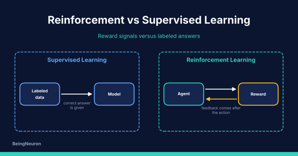
This differs from supervised learning in one key way: the targets are not fixed labels. They come from the agent’s own changing estimates and its own collected experience, which makes training less stable. For background on the networks themselves, see Multilayer Perceptron and Activation Functions.
Real-World Examples
- Game playing: DQN learned many Atari games from screen pixels and scores, and AlphaGo combined human game data with RL self-play.
- Robot control: a walking robot receives reward for forward progress and penalties for falling, usually trained first in simulation.
- Language model tuning: reinforcement learning from human feedback uses a learned preference score as the reward for refining model responses.
More applications appear in the pillar guide.
Common Misconceptions
- “Rewards are labels.” A reward says how good an outcome was, not which action was correct. The difference is explored in Reinforcement Learning vs Supervised Learning.
- “The agent knows the rules.” Model-free agents do not. They learn from outcomes. Search methods like A* search need a known map, while an RL agent in a maze can learn without one.
- “Higher immediate reward is always better.” Agents maximize return, so a small penalty now can be right.
- “RL always needs a neural network.” Tabular methods like the one above need none.
- “RL is guaranteed to find the best policy.” Tabular Q-learning has convergence guarantees under certain conditions, including enough exploration. Deep RL generally has no such guarantee.
Frequently Asked Questions
What is the difference between reward and return?
Reward is the single number received after one step. Return is the discounted sum of rewards from that point onward.
What is an episode?
An episode is one run from a starting state until a terminal state, such as reaching the maze goal. Some tasks have no natural ending and are called continuing tasks.
Does the agent learn after every step or after every episode?
Both approaches exist. Q-learning updates after each step. Monte Carlo methods wait until an episode ends and then use the full observed return.
How do I choose the learning rate and discount factor?
There is no universal value. Common starting points are small learning rates and discount factors near 0.9 to 0.99, then tune by experiment.
How long does reinforcement learning take to train?
Small tabular problems can finish in seconds. Deep RL on complex tasks often needs millions of interaction steps.
Conclusion
Reinforcement learning works through a repeating loop of observing, acting, receiving feedback, and updating. Each update moves an estimate toward the reward plus the discounted value of what comes next, and over many episodes that information spreads backward from the goal to earlier decisions. Exploration keeps the agent from settling too early, and neural networks extend the same idea to problems too large for a table. Next, learn how this differs from other learning styles in Reinforcement Learning vs Supervised Learning, or take a closer look at the learner itself in What Is an Agent in Reinforcement Learning?